Chapter: Civil : Construction Planning And Scheduling
Presenting Project Schedules

Civil - Construction Planning And Scheduling:
Presenting Project Schedules
Communicating the project schedule is a vital
ingredient in successful project management. A good presentation will greatly
ease the manager's problem of understanding the multitude of activities and
their inter-relationships. Moreover, numerous individuals and parties are
involved in any project, and they have to understand their assignments.
Graphical presentations of project schedules are particularly useful since it
is much easier to comprehend a graphical display of numerous pieces of
information than to sift through a large table of numbers. Early computer
scheduling systems were particularly poor in this regard since they produced
pages and pages of numbers without aids to the manager for understanding them.
A short example appears in Tables 2-5 and 2-6; in practice, a project summary
table would be much longer. It is extremely tedious to read a table of activity
numbers, durations, schedule times, and floats and thereby gain an
understanding and appreciation of a project schedule. In practice, producing
diagrams manually has been a common prescription to the lack of automated drafting
facilities. Indeed, it has been common to use computer programs to perform
critical path scheduling and then to produce bar charts of detailed activity
schedules and resource assignments manually. With the availability of computer
graphics, the cost and effort of producing graphical presentations has been
significantly reduced and the production of presentation aids can be automated.
Network
diagrams for projects have already been introduced. These diagrams provide a
powerful visualization of the precedence and relationships among the various
project activities. They are a basic means of communicating a project plan
among the participating planners and project monitors. Project planning is
often conducted by producing network representations of greater and greater
refinement until the plan is satisfactory.
A useful variation on project network diagrams is
to draw a time-scaled network. The activity diagrams shown in the previous
section were topological networks in that only the relationship between nodes
and branches were of interest. The actual diagram could be distorted in any way
desired as long as the connections between nodes were not changed. In
time-scaled network diagrams, activities on the network are plotted on a
horizontal axis measuring the time since project commencement. Figure 10-8
gives an example of a time-scaled activity-on-branch
diagram
for the nine activity project in Figure 10-4. In this time-scaled diagram, each
node is shown at its earliest possible time. By looking over the horizontal
axis, the time at which activity can begin can be observed. Obviously, this
time scaled diagram is produced as a display after activities are initially
scheduled by the critical path method.

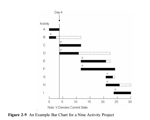
Another useful graphical representation tool is a
bar or Gantt chart illustrating the scheduled time for each activity. The bar
chart lists activities and shows their scheduled start, finish and duration. An
illustrative bar chart for the nine activity project appearing in Figure 2-4 is
shown in Figure 2-9. Activities are listed in the vertical axis of this figure,
while time since project commencement is shown along the horizontal axis.
During the course of monitoring a project, useful additions to the basic bar
chart include a vertical line to indicate the current time plus small marks to
indicate the current state of work on each activity. In Figure 2-9, a
hypothetical project state after 4 periods is shown. The small "v"
marks on each activity represent the current state of each activity.
Bar
charts are particularly helpful for communicating the current state and
schedule of activities on a project. As such, they have found wide acceptance
as a project representation tool in the field. For planning purposes, bar
charts are not as useful since they do not indicate the precedence
relationships among activities. Thus, a planner must remember or record
separately that a change in one activity's schedule may require changes to
successor activities. There have been various schemes for mechanically linking
activity bars to represent precedences, but it is now easier to use computer
based tools to represent such relationships.
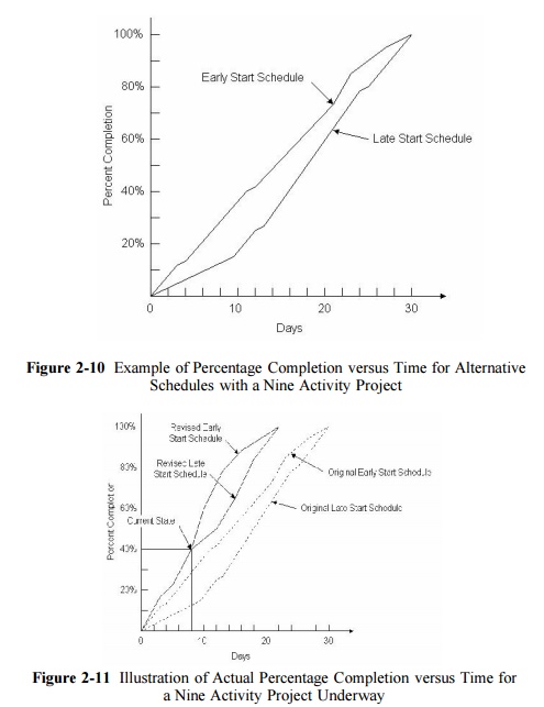
Other graphical representations are also useful in
project monitoring. Time and activity graphs are extremely useful in portraying
the current status of a project as well as the existence of activity float. For
example, Figure 2-10 shows two possible schedules for the nine activity project
described in Table 1-1 and shown in the previous figures. The first schedule
would occur if each activity was scheduled at its earliest start time, ES(i,j)
consistent with completion of the project in the minimum possible time.
With this schedule, Figure 2-10 shows the percent
of project activity completed versus time. The second schedule in Figure 2-10
is based on latest possible start times for each activity, LS(i,j). The
horizontal time difference between the two feasible schedules gives an
indication of the extent of possible float. If the project goes according to
plan, the actual percentage completion at different times should fall between
these curves. In practice, a vertical axis representing cash expenditures
rather than percent completed is often used in developing a project
representation of this type. For this purpose, activity cost estimates are used
in preparing a time versus completion graph. Separate "S-curves" may
also be prepared for groups of activities on the same graph, such as separate
curves for the design, procurement, foundation or particular sub-contractor
activities.
Time
versus completion curves are also useful in project monitoring. Not only the
history of the project can be indicated, but the future possibilities for
earliest and latest start times. For example, Figure 2-11 illustrates a project
that is forty percent complete after eight days for the nine activity example.
In this case, the project is well ahead of the original schedule; some
activities were completed in less than their expected durations. The possible
earliest and latest start time schedules from the current project status are
also shown on the figure
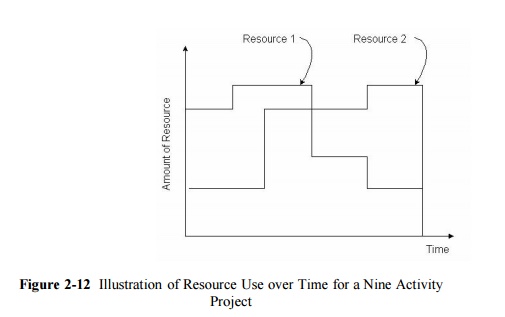
Graphs of
resource use over time are also of interest to project planners and managers.
An example of resource use is shown in Figure 2-12 for the resource of total
employment on the site of a project. This graph is prepared by summing the
resource requirements for each activity at each time period for a particular
project schedule. With limited resources of some kind, graphs of this type can
indicate when the competition for a resource is too large to accommodate; in
cases of this kind, resource constrained scheduling may be necessary as
described in Section 2.9. Even without fixed resource constraints, a scheduler
tries to avoid extreme fluctuations in the demand for labor or other resources
since these fluctuations typically incur high costs for training, hiring,
transportation, and management. Thus, a planner might alter a schedule through
the use of available activity floats so as to level or smooth out the demand
for resources. Resource graphs such as Figure 2-12 provide an invaluable
indication of the potential trouble spots and the success that a scheduler has
in avoiding them.
A common difficulty with project
network diagrams is that too much information is available for easy
presentation in a network. In a project with, say, five hundred activities,
drawing activities so that they can be seen without a microscope requires a
considerable expanse of paper. A large project might require the wall space in
a room to include the entire diagram. On a computer display, a typical
restriction is that less than twenty activities can be successfully displayed
at the same time. The problem of displaying numerous activities becomes
particularly acute when accessory information such as activity identifying
numbers or phrases, durations and resources are added to the diagram.
One practical solution to this
representation problem is to define sets of activities that can be represented
together as a single activity. That is, for display purposes, network diagrams
can be produced in which one "activity" would represent a number of
real sub-activities. For example, an activity such as "foundation
design" might be inserted in summary diagrams. In the actual project plan,
this one activity could be sub- divided into numerous tasks with their own
precedences, durations and other attributes. These sub-groups are sometimes
termed fragnets for fragments of the full network. The result of this
organization is the possibility of producing diagrams that summarize the entire
project as well as detailed representations of particular sets of activities.
The hierarchy of diagrams can also be introduced to the production of reports
so that summary reports for groups of activities can be produced. Thus,
detailed representations of particular activities such as plumbing might be
prepared with all other activities either omitted or summarized in larger,
aggregate activity representations. The CSI/MASTERSPEC activity definition
codes described in Chapter 1 provide a widely adopted example of a hierarchical
organization of this type. Even if summary reports and diagrams are prepared,
the actual scheduling would use detailed activity characteristics, of course.
An
example figure of a sub-network appears in Figure 2-13. Summary displays would
include only a single node A to represent the set of activities in the
sub-network. Note that precedence relationships shown in the master network
would have to be interpreted with care since a particular precedence might be
due to an activity that would not commence at the start of activity on the
sub-network.

The use of graphical project representations is an
important and extremely useful aid to planners and managers. Of course,
detailed numerical reports may also be required to check the peculiarities of
particular activities. But graphs and diagrams provide an invaluable means of
rapidly communicating or understanding a project schedule. With computer based
storage of basic project data, graphical output is readily obtainable and
should be used whenever possible.
Finally,
the scheduling procedure described in Section 2.3 simply counted days from the
initial starting point. Practical scheduling programs include a calendar
conversion to provide calendar dates for scheduled work as well as the number
of days from the initiation of the project. This conversion can be accomplished
by establishing a one-to-one correspondence between project dates and calendar
dates. For example, project day 2 would be May 4 if the project began at time 0
on May 2 and no holidays intervened. In this calendar conversion, weekends and
holidays would be excluded from consideration for scheduling, although the
planner might overrule this feature. Also, the number of work shifts or working
hours in each day could be defined, to provide consistency with the time units
used is estimating activity durations. Project reports and graphs would
typically use actual calendar days.
Related Topics