Estimating Activity Durations

Construction Planning:

Estimating Activity Durations

In most scheduling procedures, each work activity has associated time duration. These durations are used extensively in preparing a schedule. For example, suppose that the durations shown in Table 9-3 were estimated for the project diagrammed in Figure 1-0. The entire set of activities would then require at least 3 days, since the activities follow one another directly and require a total of 1.0 + 0.5 + 0.5 + 1.0 = 3 days. If another activity proceeded in parallel with this sequence, the 3 day minimum duration of these four activities is unaffected. More than 3 days would be required for the sequence if there was a delay or a lag between the completion of one activity and the start of another.

All formal scheduling procedures rely upon estimates of the durations of the various project activities as well as the definitions of the predecessor relationships among tasks. The variability of an activity's duration may also be considered. Formally, the probability distribution of an activity's duration as well as the expected or most likely duration may be used in scheduling. A probability distribution indicates the chance that particular activity duration will occur. In advance of actually doing a particular task, we cannot be certain exactly how long the task will require.

A straightforward approach to the estimation of activity durations is to keep historical records of particular activities and rely on the average durations from this experience in making new duration estimates. Since the scopes of activities are unlikely to be identical between different projects, unit productivity rates are typically employed for this purpose. For example, the duration of an activity D_ij

such as concrete formwork assembly might be estimated as:

Dv = Ag / FgNg

Where A_ij is the required formwork area to assemble (in square yards), P_ij is the average productivity of a standard crew in this task (measured in square yards per hour), and N_ij is the number of crews assigned to the task. In some organizations, unit production time, T_ij, is defined as the time

required to complete a unit of work by a standard crew (measured in hours per square yards) is used as a productivity measure such that T_ij is a reciprocal of P_ij.

A formula such as Eq. (1.1) can be used for nearly all construction activities. Typically, the required quantity of work, A_ij is determined from detailed examination of the final facility design. This

quantity-take-off to obtain the required amounts of materials, volumes, and areas is a very common process in bid preparation by contractors. In some countries, specialized quantity surveyors provide the information on required quantities for all potential contractors and ^{the owner. The number of crews} working, N_ij, is decided by the planner. In many cases, the number or amount of resources applied to

particular activities may be modified in light of the resulting project plan and schedule. Finally, some estimate of the expected work productivity, P_ij must be provided to apply _{Equation (1.1). As with cost} factors, commercial services can provide average productivity figures for many standard activities of this sort. Historical records in a firm can also provide data for estimation of productivities.

The calculation of a duration as in Equation (9.1) is only an approximation to the actual activity duration for a number of reasons. First, it is usually the case that peculiarities of the project make the accomplishment of a particular activity more or less difficult. For example, access to the forms in a particular location may be difficult; as a result, the productivity of assembling forms may be lower than the average value for a particular project. Often, adjustments based on engineering judgment are made to the calculated durations from Equation (9.1) for this reason.

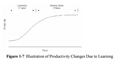
In addition, productivity rates may vary in both systematic and random fashions from the average. An example of systematic variation is the effect of learning on productivity. As a crew becomes familiar with an activity and the work habits of the crew, their productivity will typically improve. Figure 9-7 illustrates the type of productivity increase that might occur with experience; this curve is called a learning curve. The result is that productivity P_ij is a function of the duration of an activity or project. A

common construction example is that the assembly of floors in a building might go faster at higher levels due to improved productivity even though the transportation time up to the active construction area is longer. Again, historical records or subjective adjustments might be made to represent learning curve variations in average productivity.

Random factors will also influence productivity rates and make estimation of activity durations uncertain. For example, a scheduler will typically not know at the time of making the initial schedule how skillful the crew and manager will be that are assigned to a particular project. The productivity of a skilled designer may be many times that of an unskilled engineer. In the absence of specific knowledge, the estimator can only use average values of productivity.

Weather effects are often very important and thus deserve particular attention in estimating durations. Weather has both systematic and random influences on activity durations. Whether or not a rainstorm will come on a particular day is certainly a random effect that will influence the productivity of many activities. However, the likelihood of a rainstorm is likely to vary systematically from one month or one site to the next. Adjustment factors for inclement weather as well as meteorological records can be used to incorporate the effects of weather on durations. As a simple example, an activity might require ten days in perfect weather, but the activity could not proceed in the rain. Furthermore, suppose that rain is expected ten percent of the days in a particular month. In this case, the expected activity duration is eleven days including one expected rain day.

Finally, the use of average productivity factors themselves cause problems in the calculation presented in Equation (1.1). The expected value of the multiplicative reciprocal of a variable is not exactly equal to the reciprocal of the variable's expected value. For example, if productivity on an activity is either six in good weather (ie., P=6) or two in bad weather (ie., P=2) and good or bad weather is equally likely, then the expected productivity is P = (6)(0.5) + (2) (0.5) = 4, and the reciprocal of expected productivity is 1/4. However, the expected reciprocal of productivity is E[1/P] = (0.5)/6 + (0.5)/2 = 1/3. The reciprocal of expected productivity is 25% less than the expected value of the reciprocal in this case! By representing only two possible productivity values, this example represents an extreme case, but it is always true that the use of average productivity factors in Equation (1.1) will result in optimistic estimates of activity durations. The use of actual averages for the reciprocals of productivity or small adjustment factors may be used to correct for this non-linearity problem.

The simple duration calculation shown in Equation (1.1) also assumes an inverse linear relationship between the number of crews assigned to an activity and the total duration of work. While this is a reasonable assumption in situations for which crews can work independently and require no special coordination, it need not always be true. For example, design tasks may be divided among numerous architects and engineers, but delays to insure proper coordination and communication increase as the number of workers increase. As another example, insuring a smooth flow of material to all crews on a site may be increasingly difficult as the number of crews increase. In these latter cases, the relationship between activity duration and the number of crews is unlikely to be inversely proportional as shown in Equation (1.1). As a result, adjustments to the estimated productivity from Equation (1.1) must be made. Alternatively, more complicated functional relationships might be estimated between duration and resources used in the same way that nonlinear preliminary or conceptual cost estimate models are prepared.

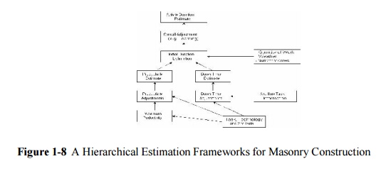
One mechanism to formalize the estimation of activity durations is to employ a hierarchical estimation framework. This approach decomposes the estimation problem into component parts in which the higher levels in the hierarchy represent attributes which depend upon the details of lower level adjustments and calculations. For example, Figure 1-8 represents various levels in the estimation of the duration of masonry construction. At the lowest level, the maximum productivity for the activity is estimated based upon general work conditions. Table 1-4 illustrates some possible maximum productivity values that might be employed in this estimation. At the next higher level, adjustments to these maximum productivities are made to account for special site conditions and crew compositions; table 1-5 illustrates some possible adjustment rules. At the highest level, adjustments for overall effects such as weather are introduced. Also shown in Figure 1-8 are nodes to estimate down or unproductive time associated with the masonry construction activity. The formalization of the estimation process illustrated in Figure 1-8 permits the development of computer aids for the estimation process or can serve as a conceptual framework for a human estimator.

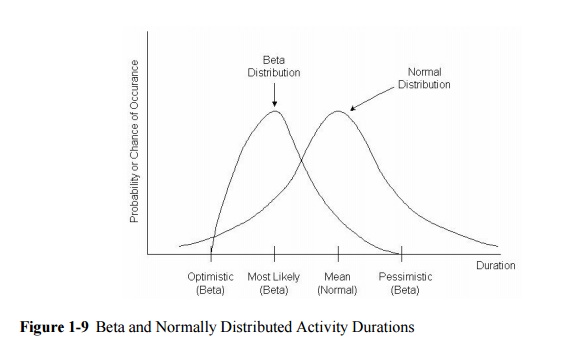
In addition to the problem of estimating the expected duration of an activity, some scheduling procedures explicitly consider the uncertainty in activity duration estimates by using the probabilistic distribution of activity durations. That is, the duration of a particular activity is assu med to be a random variable that is distributed in a particular fashion. For example, an activity duration might be assumed to be distributed as a normal or a beta distributed random variable as illustrated in Figure 9-9. This figure shows the probability or chance of experiencing a particular activity duration based on a probabilistic distribution. The beta distribution is often used to characterize activity durations, since it can have an absolute minimum and an absolute maximum of possible duration times. The normal distribution is a good approximation to the beta distribution in the center of the distribution and is easy to work with, so it is often used as an approximation.

If a standard random variable is used to characterize the distribution of activity durations, then only a few parameters are required to calculate the probability of any particular duration. Still, the estimation problem is increased considerably since more than one parameter is required to characterize most of the probabilistic distribution used to represent activity durations. For the beta distribution, three or four parameters are required depending on its generality, whereas the normal distribution requires two parameters.

As an example, the normal distribution is characterized by two parameters,  and  representing the average duration and the standard deviation of the duration, respectively. Alternatively, the variance of the distribution  could be used to describe or characterize the

variability of duration times; the variance is the value of the standard deviation multiplied by itself. From historical data, these two parameters can be estimated as:

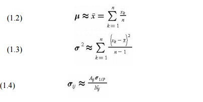
where we assume that n different observations x_k of the random variable x are available. This estimation process might be applied to activity durations directly (so that x_k would be a record of an activity duration D_ij on a past project) or to the estimation of the distribution of productivities (so that x_k would be a record of the productivity in an activity P_i) on a past project) which, in turn, is used to

estimate durations using Equation (1.4). If more accuracy is desired, the estimation equations for mean and standard deviation, Equations (1.2) and (1.3) would be used to estimate the mean and standard deviation of the reciprocal of productivity to avoid non-linear effects. Using estimates of productivities, the standard deviation of activity duration would be calculated as:

where Ro (p) is the estimated standard deviation of the reciprocal of productivity that is calculated from Equation (1.3) by substituting 1/P for x.