Point and Interval Estimation

Point and Interval Estimation:

To estimate an unknown parameter of the population, concept of theory of estimation is used.There are two types of estimation namely,

1. Point estimation

2. Interval estimation

1. Point Estimation

When a single value is used as an estimate, the estimate is called a point estimate of the population parameter. In other words, an estimate of a population parameter given by a single number is called as point estimation.

For example

(i) 55 is the mean mark obtained by a sample of 5 students randomly drawn from a class of 100 students is considered to be the mean marks of the entire class. This single value 55is a point estimate.

(ii) 50 kg is the average weight of a sample of 10 students randomly drawn from a class of 100 students is considered to be the average weight of the entire class. This single value 50 is a point estimate.

Note

The sample mean () is the sample statistic used as an estimate of population mean (μ)

Instead of considering, the estimated value of the population parameter to be a single value, we might consider an interval for estimating the value of the population parameter. This concept is known as interval estimation and is explained below.

2. Interval Estimation

Generally, there are situations where point estimation is not desirable and we are interested in finding limits within which the parameter would be expected to lie is called an interval estimation.

For example,

If T is a good estimator of θ with standard error s then, making use of general property of the standard deviations, the uncertainty in T, as an estimator of q, can be expressed by statements like “ We are about 95% certain that the unknown q, will lie somewhere between T-2s and T+2s”, “we are almost sure that q will in the interval ( T-3s and T+3s)” such intervals are called confidence intervals and is explained below.

Confidence interval

After obtaining the value of the statistic ‘t’ (sample) from a given sample, Can we make some reasonable probability statements about the unknown population parameter ‘ θ’ ?. This question is very well answered by the technique of Confidence Interval. Let us choose a small value of a which is known as level of significance(1% or 5%) and determine two constants say, c₁ and c₂ such that P (c₁ < θ < c ₂ |t) = 1 − α .

The quantities c₁ and c₂, so determined are known as the Confidence Limits and the interval [c₁,c₂] within which the unknown value of the population parameter is expected to lie is known as Confidence Interval. (1− a) is called as confidence coefficient.

Confidence Interval for the population mean for Large Samples (when  is known)

If we take repeated independent random samples of size n from a population with an unknown mean but known standard deviation, then the probability that the true population mean μ will fall in the following interval is (1− α) i.e

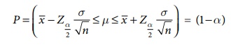
So, the confidence interval for population mean (μ), when standard deviation (σ) is known and is given by

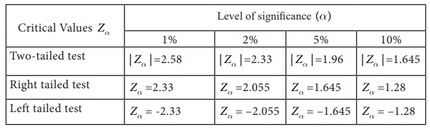
For the computation of confidence intervals and for testing of significance, the critical values

Z_a  at the different level of significance is given in the following table:

Normal Probability Table

The calculation of confidence interval is illustrated below.

Example 8.11

A machine produces a component of a product with a standard deviation of 1.6 cm in length. A random sample of 64 componentsvwas selected from the output and this sample has a mean length of 90 cm. The customer will reject the part if it is either less than 88 cm or more than 92 cm. Does the 95% confidence interval for the true mean length of all the components produced ensure acceptance by the customer?

Solution:

Here μ is the mean length of the components in the population.

The formula for the confidence interval is

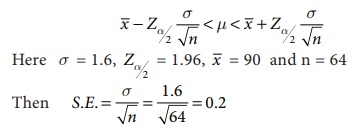
Therefore, 90 − (1.96 × 0.2) ≤ μ ≤ 90 + (1.96 × 0.2)

(89.61 ≤ μ ≤ 90.39)

This implies that the probability that the true value of the population mean length of the components will fall in this interval (89.61,90.39) at 95% . Hence we concluded that 95% confidence interval ensures acceptance of the component by the consumer.

Example 8.12

A sample of 100 measurements at breaking strength of cotton thread gave a mean of 7.4 and a standard deviation of 1.2 gms. Find 95% confidence limits for the mean breaking strength of cotton thread.

Solution:

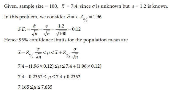
This implies that the probability that the true value of the population mean breaking strength of the cotton threads will fall in this interval (7.165,7.635) at 95% .

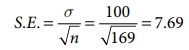
Example 8.13

The mean life time of a sample of 169 light bulbs manufactured by a company is found to be 1350 hours with a standard deviation of 100 hours. Establish 90% confidence limits within which the mean life time of light bulbs is expected to lie.

Solution:

Given: n = 169,  = 1350 hours, s = 100 hours, since the level of significance is (100-90)% =10% thus a is 0.1, hence the significant value at 10% is Za/2 = 1.645

Hence 90% confidence limits for the population mean are

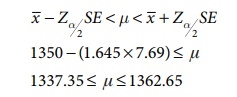
Hence the mean life time of light bulbs is expected to lie between the interval (1337.35, 1362.65)