Applications of differentiation in business and economics - Elasticity | 11th Business Mathematics and Statistics(EMS) : Chapter 6 : Applications of Differentiation
Chapter: 11th Business Mathematics and Statistics(EMS) : Chapter 6 : Applications of Differentiation
Elasticity
Elasticity
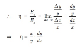
Elasticity ŌĆś╬ĘŌĆÖ of the function y = f (x ) at a
point x is defined as the limiting
case of ratio of the relative change in y
to the relative change in x.
(i) Price elasticity of demand
Price elasticity of demand is the
degree of responsiveness of quantity demanded to a change in price.
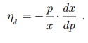
If x is demand and p is unit
price of the demand function x = f(p),
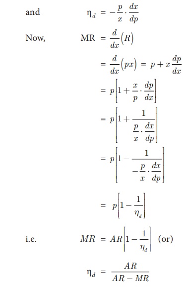
then the elasticity of demand with respect to the price is defined as hd =
(ii) Price elasticity of supply :
Price elasticity of supply is the
degree of responsiveness of quantity supplied to a change in price.
If x is supply and p is unit price of the supply function x = g(p), then the elasticity of supply with respect to the price is defined as hs

Some important results on price elasticity
(i) If |
╬Ę |>1, then the quantity demand or supply is said to be elastic.
(ii) If |
╬Ę |=1, then the quantity demand or supply is said to be unit elastic.
(iii) If | ╬Ę |<1, then the
quantity demand or supply is said to be inelastic.
Remarks:
(i) Elastic : A quantity demand
or supply is elastic when its quantity responds greatly to changes in its
price.
Example: Consumption of onion and
its price.
(ii) Inelastic : A quantity
demand or supply is inelastic when its quantity responds very little to changes
in its price.
Example: Consumption of rice and its price.
(iii) Unit elastic : A quantity
demand or supply is unit elastic when its quantity responds as the same ratio
as changes in its price.
Relationship among Marginal revenue [MR], Average revenue [AR] and Elasticity of demand[╬Ęd].
We know that R(x)=px
Example 6.1
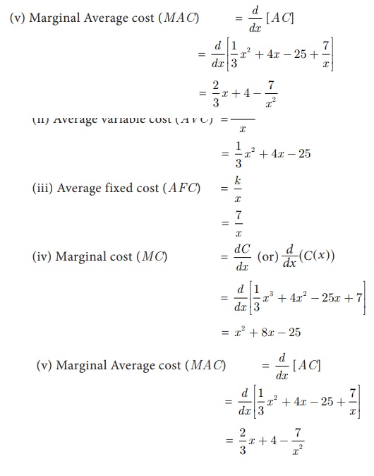
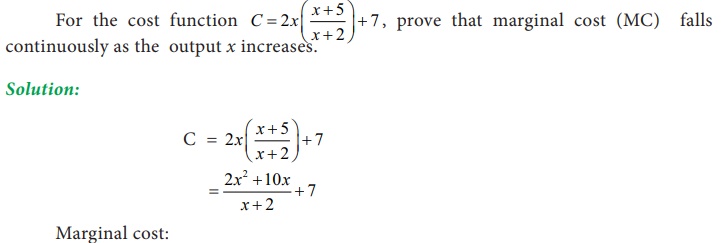
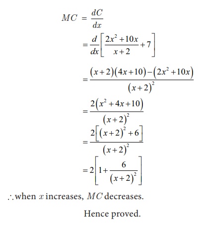
The total cost function for the
production of x units of an item is
given by
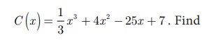
(i) Average cost
(ii) Average variable cost
(iii) Average fixed cost
(iv) Marginal cost and
(v) Marginal Average cost
Solution:
Example 6.2
The total cost C in Rupees of making x units of product is C (x ) = 50 + 4x + 3ŌłÜx . Find
the marginal cost of the product at 9 units of output.
Solution:
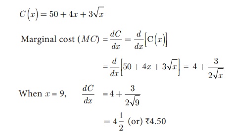
MC is Ōé╣ 4.50 , when the level of output is 9 units.
Example 6.3
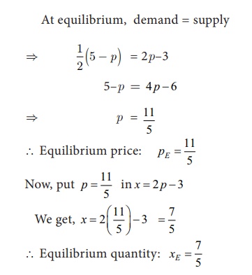
Find the equilibrium price and
equilibrium quantity for the following demand and supply functions.
Demand : x = 1/2 (5 ŌłÆ p) and
Supply : x = 2pŌĆō3
Solution:
Example 6.4
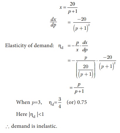
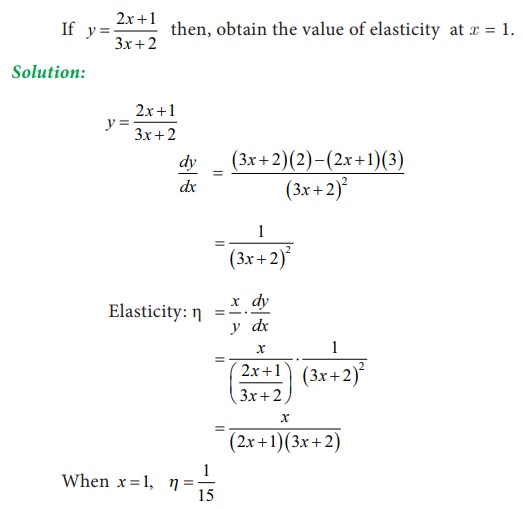
For the demand function x=20/P+1, find the elasticity of demand
with respect to price at a point p =
3. Examine whether the demand is elastic at p
= 3.
Solution:
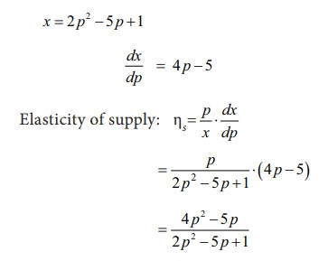
Example 6.5
Find the elasticity of supply for
the supply function x = 2p2 - 5 p + 1
Solution:
Example 6.6
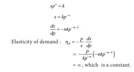
Example 6.7
A demand function is given by xpn = k where n and k are constants. Prove that elasticity
of demand is always constant.
Solution:
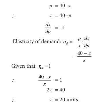
Example 6.8
For the given demand function p = 40ŌĆōx, find the value of the output when ╬Ęd =1
Solution:
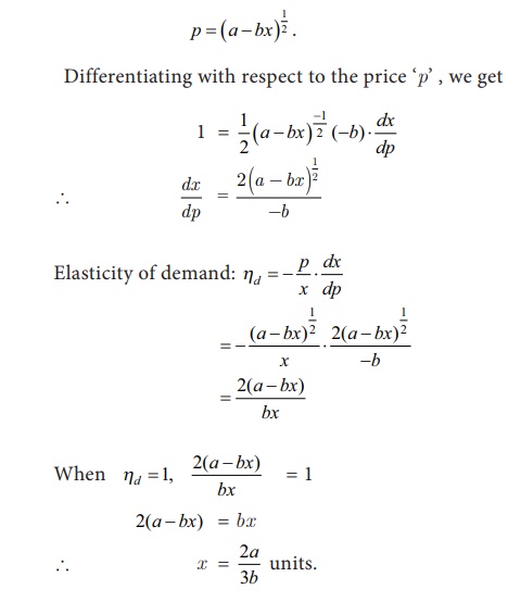
Example 6.9
Find the elasticity of demand in
terms of x for the demand law p = (a-bx)1/2 . Also find the
values of x when elasticity of demand
is unity.
Solution:
Example 6.10
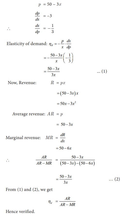
Verify the relationship of
elasticity of demand, average revenue and marginal revenue for the demand law p = 50 - 3x .
Solution:
Example 6.11
Find the elasticity of supply for
the supply law x = p / p+5 when p = 20
and interpret your result.
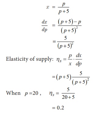
Interpretation:
┬Ę
z If the price increases by 1% from p = Ōé╣ 20, then
the quantity of supply increases by 0.2% approximately.
┬Ę
z If the price decreases by 1% from p = Ōé╣ 20, then
the quantity of supply decreases by 0.2% approximately.
Example 6.12
Example 6.13
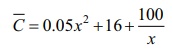 is the manufacturerŌĆÖs average cost function. What is the marginal cost when 50 units are produced and interpret your result.
Solution:
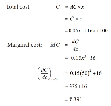
Interpretation:
If the production level is
increased by one unit from x = 50,
then the cost of additional unit is approximately equal to Ōé╣ 391.
Example 6.14
For the function y x3+19,
find the values of x when its
marginal value is equal to 27.
Solution:
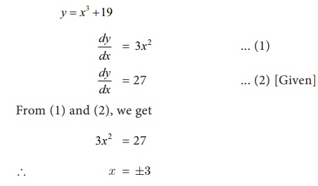
Example 6.15
The demand function for a
commodity is p = 4/x,where
p is unit price. Find the
instantaneous rate of change of demand with respect to price at p=4. Also interpret your result.
Solution:
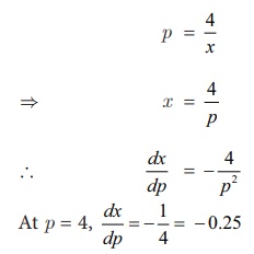
Rate of change of demand with
respect to the price at p
= Ōé╣ 4 is ŌłÆ 0.25
Interpretation:
When the price increases by 1%
from the level of p = Ōé╣ 4, the demand decreases (falls)
by 0.25%
Example 6.16
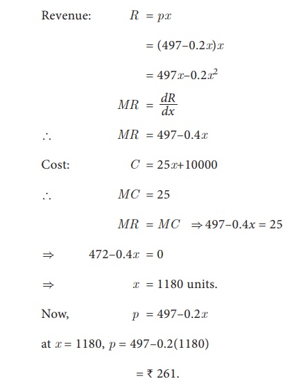
The demand and the cost function
of a firm are p = 497-0.2x and C = 25x+10000
respectively. Find the output level and price at which the profit is maximum.
Solution:
We know that profit is maximum
when marginal revenue [MR] = marginal cost [MC].
Revenue: R = px
Example 6.17
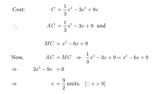
The cost function of a firm is C = 1/3 x3 ŌłÆ 3x2 + 9x . Find the level of output (x>0)
when average cost is minimum.
Solution:
We know that average cost [AC] is
minimum when average cost [AC] = marginal cost [MC].

Related Topics