Shapes of atomic orbitals

Shapes of atomic orbitals:

The solution to SchrÖdinger equation gives the permitted energy values called eigen values and the wave functions corresponding to the eigen values are called atomic orbitals. The solution (Ψ) of the SchrÖdinger wave equation for one electron system like hydrogen can be represented in the following form in spherical polar coordinates r, θ, φ as,

Ψ (r, θ, φ) = R(r).f(θ).g(φ) ------                                                                                      (2.15)

(where R(r) is called radial wave function, other two functions are called angular wave functions)

As we know, the Ψ itself has no physical meaning and the square of the wave function |Ψ|2 is related to the probability of finding the electrons within a given volume of space. Let us analyse how |Ψ|2 varies with the distance from nucleus (radial distribution of the probability) and the direction from the nucleus (angular distribution of the probability).

Radial distribution function:

Consider a single electron of hydrogen atom in the ground state for which the quantum numbers are n=1 and l=0. i.e. it occupies 1s orbital. The plot of R(r)2 versus r for 1s orbital is given in Figure 2.3

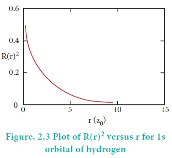
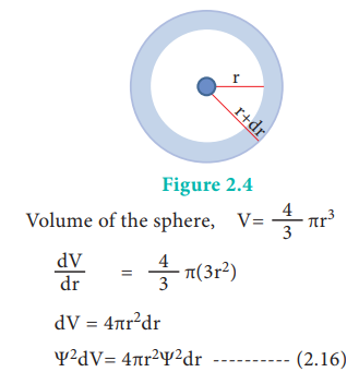
The graph shows that as the distance between the electron and the nucleus decreases, the probability of finding the electron increases. At r=0, the quantity R(r)2 is maximum i.e. The maximum value for |Ψ|2 is at the nucleus. However, probability of finding the electron in a given spherical shell around the nucleus is important. Let us consider the volume (dV) bounded by two spheres of radii r and r+dr.

The plot of 4Ï€r2Ψ2 versus r is given below.

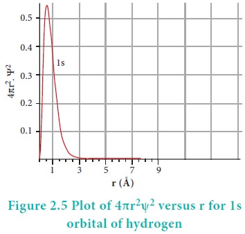
The above plot shows that the maximum probability occurs at distance of 0.52 Ã… from the nucleus. This is equal to the Bohr radius. It indicates that the maximum probability of finding the electron around the nucleus is at this distance. However, there is a probability to find the electron at other distances also. The radial distribution function of 2s, 3s, 3p and 3d orbitals of the hydrogen atom are represented as follows.

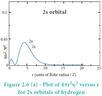
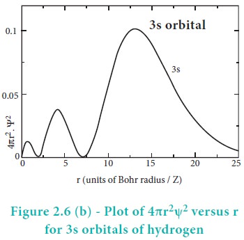
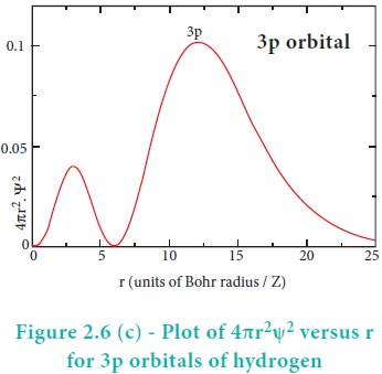
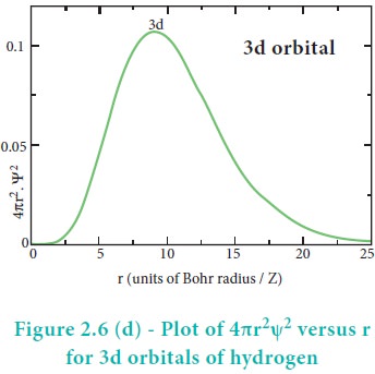
For 2s orbital, as the distance from nucleus r increases, the probability density first increases, reaches a small maximum followed by a sharp decrease to zero and then increases to another maximum, after that decreases to zero. The region where this probability density function reduces to zero is called nodal surface or a radial node. In general, it has been found that ns-orbital has (n–1) nodes. In other words, number of radial nodes for 2s orbital is one, for 3s orbital it is two and so on. The plot of 4Ï€r2ψ2 versus r for 3p and 3d orbitals shows similar pattern but the number of radial nodes are equal to(n-l-1) (where n is principal quantum number and l is azimuthal quantum number of the orbital).

Angular distribution function:

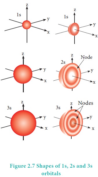
The variation of the probability of locating the electron on a sphere with nucleus at its centre depends on the azimuthal quantum number of the orbital in which the electron is present. For 1s orbital, l=0 and m=0. f(θ) = 1/√2 and g(φ) = 1/√2π. Therefore, the angular distribution function is equal to 1/2√π. i.e. it is independent of the angle θ and Hence, the probability of finding the electron is independent of the direction from the nucleus. The shape of the s orbital is spherical as shown in the figure 2.7

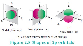
For p orbitals l=1 and the corresponding m values are -1, 0 and +1. The angular distribution functions are quite complex and are not discussed here. The shape of the p orbital is shown in Figure 2.8. The three different m values indicates that there are three different orientations possible for p orbitals. These orbitals are designated as px, py and pz and the angular distribution for these orbitals shows that the lobes are along the x, y and z axis respectively. As seen in the Figure 2.8 the 2p orbitals have one nodal plane.

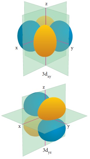
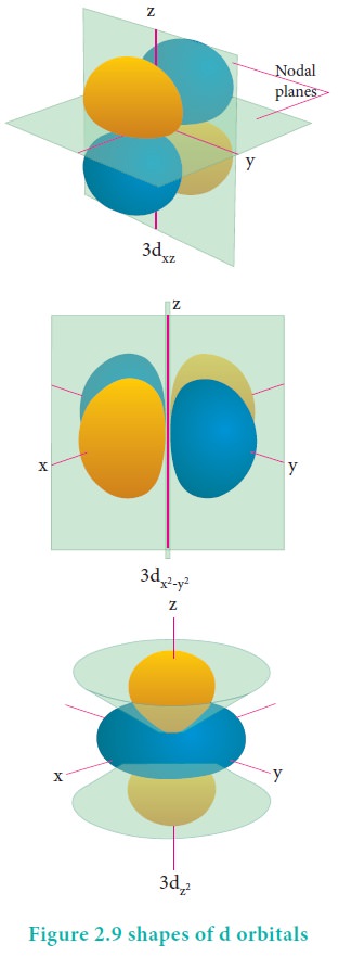
For ‘d’  orbital  l =  2   and  the corresponding m values are -2, -1, 0 +1,+2. The shape of the d orbital looks like a 'clover leaf '. The five m values give rise to five d orbitals namely dxy , dyz, dzx, dx2, dz2, and dz2. The 3d orbitals contain two nodal planes as shown in Figure 2.9.

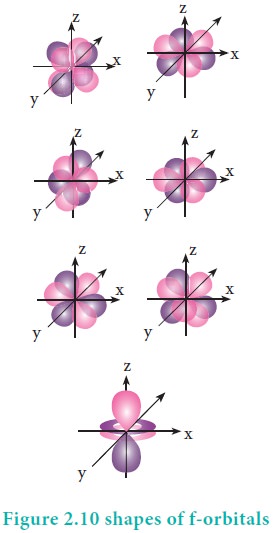
For 'f ' orbital, l = 3 and the m values are -3, -2,-1, 0, +1, +2, +3 corresponding to seven f orbitals fz3, fxz2, fyz2, fxyz, fz(x2−y2), fx(x2−3y2), fy(3x2−y2), which are shown in Figure 2.10. There are 3 nodal planes in the f-orbitals.