Parallelizing the basic solver using MPI

Parallelizing the basic solver using MPI

With our composite tasks corresponding to the individual particles, it’s fairly straight-forward to parallelize the basic algorithm using MPI. The only communication among the tasks occurs when we’re computing the forces, and, in order to compute the forces, each task/particle needs the position and mass of every other particle. MPI_Allgather is expressly designed for this situation, since it collects on each process the same information from every other process. We’ve already noted that a block distribution will probably have the best performance, so we should use a block mapping of the particles to the processes.

In the shared-memory implementations, we collected most of the data associated with a single particle (mass, position, and velocity) into a single struct. However, if we use this data structure in the MPI implementation, we’ll need to use a derived datatype in the call to MPI_Allgather, and communications with derived datatypes tend to be slower than communications with basic MPI types. Thus, it will make more sense to use individual arrays for the masses, positions, and velocities. We’ll also need an array for storing the positions of all the particles. If each process has sufficient memory, then each of these can be a separate array. In fact, if memory isn’t a problem, each process can store the entire array of masses, since these will never be updated and their values only need to be communicated during the initial setup.

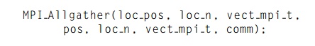
On the other hand, if memory is short, there is an “in-place” option that can be used with some MPI collective communications. For our situation, suppose that the array pos can store the positions of all n particles. Further suppose that vect mpi t is an MPI datatype that stores two contiguous doubles. Also suppose that n is evenly divisible by comm._sz and loc_n = n/comm._sz. Then, if we store the local positions in a separate array, loc pos, we can use the following call to collect all of the positions on each process:

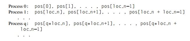
If we can’t afford the extra storage for loc pos, then we can have each process q store its local positions in the qth block of pos. That is, the local positions of each process should be stored in the appropriate block of each process’ pos array:

With the pos array initialized this way on each process, we can use the following call to MPI Allgather:

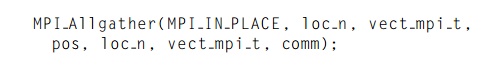
In this call, the first loc_n and vect_mpi_t arguments are ignored. However, it’s not a bad idea to use arguments whose values correspond to the values that will be used, just to increase the readability of the program.

In the program we’ve written, we made the following choices with respect to the data structures:

._. Each process stores the entire global array of particle masses.

_. Each process only uses a single n-element array for the positions.

Each process uses a pointer loc_pos that refers to the start of its block of pos. Thus, on process, 0 local_pos = pos, on process 1 local_pos = pos + loc_n, and, so on.

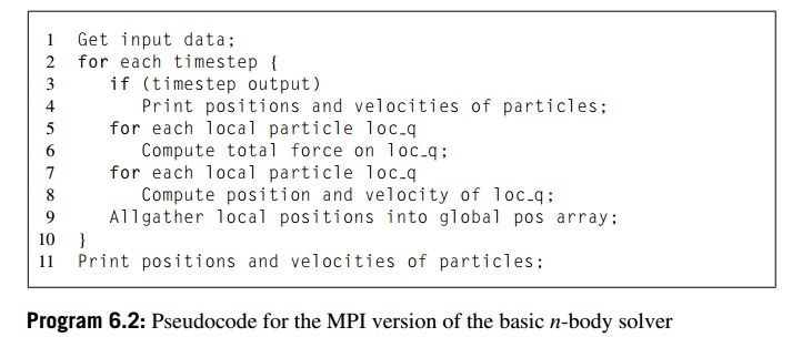
With these choices, we can implement the basic algorithm with the pseudocode shown in Program 6.2. Process 0 will read and broadcast the command line argu-ments. It will also read the input and print the results. In Line 1, it will need to distribute the input data. Therefore, Get input data might be implemented as follows:

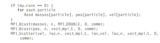
So process 0 reads all the initial conditions into three n-element arrays. Since we’re storing all the masses on each process, we broadcast masses. Also, since each process

will need the global array of positions for the first computation of forces in the main for loop, we just broadcast pos. However, velocities are only used locally for the updates to positions and velocities, so we scatter vel.

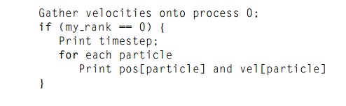
Notice that we gather the updated positions in Line 9 at the end of the body of the outer for loop of Program 6.2. This insures that the positions will be avail-able for output in both Line 4 and Line 11. If we’re printing the results for each timestep, this placement allows us to eliminate an expensive collective communica-tion call: if we simply gathered the positions onto process 0 before output, we’d have to call MPI_Allgather before the computation of the forces. With this organization of the body of the outer for loop, we can implement the output with the following pseudocode: