Slip Line Theory

SlipLine Theory

Only at points where we know the orientation of the principal stresses do we know the orientation of the slip surface to be +- (45 + ϕ/2) to the direction of σ₁. We often know the principal orientation at boundaries, but seldom anywhere else. As the stresses change throughout the field in some fashion so do the isoclinics and the slip surface must, therefore, in general be curved.

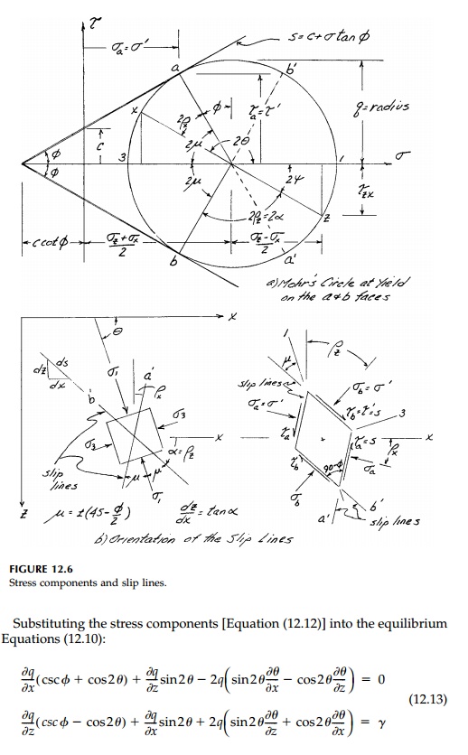
To determine the shape or characteristic of the slipline field we must solve the basic equations in terms of geometric parameters. Rewriting the MohrCoulomb criterion in terms of a general stress state:

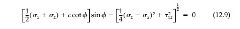
where, from Figure 12.6a each of the two terms equals the radius of Mohr’s Circle, q. We also have the equilibrium equations:

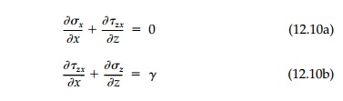
where the unit weight is assumed to be the only body force.

It would appear that with three equations, [Equations (12.9), (12.10a), and (12.10b)], the determination of the three unknown stress components is determinate. However, this is not really true since the yield Equation (12.9) is only true on the slip surfaces for which we do not know the shape or critical location.

The two slip lines (or characteristic lines) are inclined at an angle 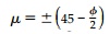 to the direction of the maximum principal compressive stress σ1. Since Mohr’s Circle gives the orientation of the normal to the surface on which the stresses act, the orientation of the surface itself is at 90� o or 180� o on Mohr’s Circle. From Figure 12.6b, the equations for the slip lines are then:

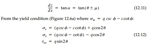
and the stress components producing potential slip are expressed in terms of the invariant q and the isoclinic angle θ.

and, from the definition of a total derivative, trigonometric identities, and Equation (12.11), these can be reduced to

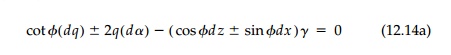
This equation, obtained by Kötter in 1888 expresses, in differential form, the variation of the critical stress state, q, on the slip surface as the orientation  α of the slip surface changes. It can be written in terms of the various components of the critical state which may be useful in different cases. On the slip planes where Mohr’s Circle touches the failure envelope:

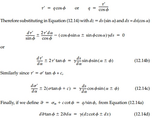
which is the version often used for integration along a slip line.

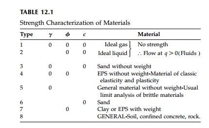
Various combinations of the three material properties used to characterize yield of a MohrCoulomb material are summarized in Table 12.1. If we assume a yield plateau and thus eliminate strain effects, these properties will not change as the yield area spreads to form a collapse mechanism (the slip surface) at the limit load.

In the next sections we will discuss a few simple cases where Equation (12.14) can be integrated. With the stress boundary conditions, it may be possible then to determine the shape of the critical slip surface and the stresses on the slip surface at collapse. Solutions for difficult boundary loads and for the general case where ϕ, c, or ψ are not neglected can sometimes be obtained by a shooting technique called  “the method of characteristics” where Equation (12.14)

is numerically integrated by finite differences starting from one boundary and working in increments, which can be arbitrarily small, to the other boundary. Results from this method will be referred to but not derived. Some observations on the “method of characteristics” or “the slipline method” are included in the final section.