Chapter: Data Warehousing and Data Mining : Association Rule Mining and Classification
Mining Various Kinds of Association Rules
Mining Various Kinds of Association Rules
1. Mining Multilevel Association Rules
For many applications, it is difficult to find strong associations among data items at low or primitive levels of abstraction due to the sparsity of data at those levels. Strong associations discovered at high levels of abstraction may represent commonsense knowledge.
. Therefore,
data mining systems should provide capabilities for mining association rules at
multiple levels of abstraction, with sufficient flexibility for easy traversal
among different abstraction spaces.
Let’s
examine the following example.
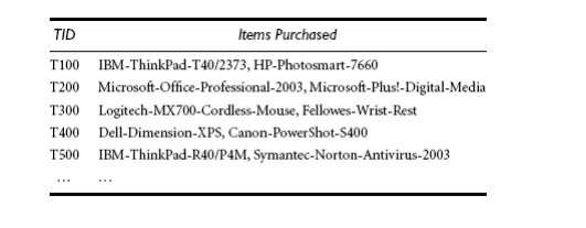
Mining
multilevel association rules. Suppose we are given the task-relevant set of
transactional data in Table for sales in an AllElectronics
store, showing the items purchased for each transaction.
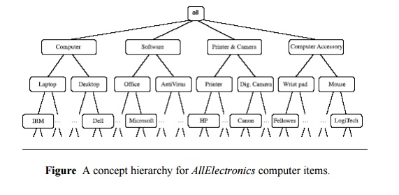
The
concept hierarchy for the items is shown in Figure . A concept hierarchy
defines a sequence of mappings from a set of low-level concepts to higher
level, more general concepts. Data can be generalized by replacing low-level
concepts within the data by their higher-level concepts, or ancestors, from a concept hierarchy.
Association
rules generated from mining data at multiple levels of abstraction are called
multiple-level or multilevel association rules. Multilevel association rules
can be mined efficiently using concept hierarchies under a support-confidence
framework. In general, a top-down strategy is employed, For each level, any
algorithm for discovering frequent itemsets may be used, such as Apriori or its
variations.
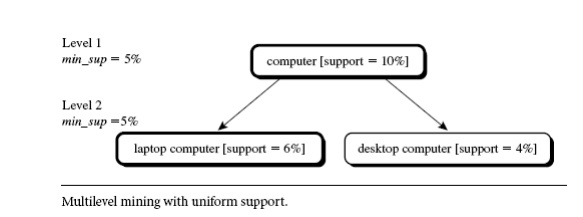
Using uniform minimum support for
all levels (referred to as uniform support): The same minimum support threshold is used when mining at each level
of abstraction. For example, in Figure 5.11, a minimum support threshold of 5%
is used throughout (e.g., for mining from
“computer” down to “laptop computer”). Both “computer” and “laptop computer” are found to
be frequent, while “desktop computer”
is not.
When a
uniform minimum support threshold is used, the search procedure is simplified.
The method is also simple in that users are required to specify only one
minimum support threshold. An Apriori-like optimization technique can be
adopted, based on the knowledge that an ancestor is a superset of its
descendants: The search avoids examining itemsets containing any item whose
ancestors do not have minimum support.
Using
reduced minimum support at lower levels (referred to as reduced support): Each level of abstraction has its own
minimum support threshold. The deeper the level of abstraction, the smaller the
corresponding threshold is. For example, in Figure, the minimum support
thresholds for levels 1 and 2 are 5% and 3%, respectively. In this way, “computer,” “laptop computer,” and
“desktop computer” are all considered frequent.
Using
item or group-based minimum support (referred to as group-based support):
Because
users or experts often have insight as to which groups are more important than
others, it is sometimes more desirable to set up user-specific, item, or group
based minimal support thresholds when mining multilevel rules. For example, a
user could set up the minimum support thresholds based on product price, or on
items of interest, such as by setting particularly low support thresholds for laptop computers and flash drives in order to pay particular
attention to the association patterns containing items in these categories.
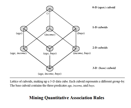
2. Mining Multidimensional Association Rules from Relational Databases
and Data Warehouses
We have
studied association rules that imply a single predicate, that is, the predicate
buys. For instance, in mining our AllElectronics database, we may discover
the Boolean association rule
Following
the terminology used in multidimensional databases, we refer to each distinct
predicate in a rule as a dimension. Hence, we can refer to Rule above as a
single dimensional or intra dimensional association rule because it contains a
single distinct predicate (e.g., buys)with
multiple occurrences (i.e., the predicate occurs more than once within the
rule). As we have seen in the previous sections of this chapter, such rules are
commonly mined from transactional data.
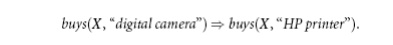
Considering
each database attribute or warehouse dimension as a predicate, we can therefore
mine association rules containing multiple
predicates, such as
Association
rules that involve two or more dimensions or predicates can be referred to as
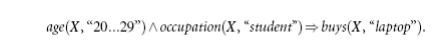
multidimensional association rules. Rule above contains three predicates (age, occupation, and buys), each of which occurs only once in the rule. Hence, we say
that it has no repeated predicates. Multidimensional
association rules with no repeated predicates are called inter dimensional
association rules. We can also mine multidimensional association rules with
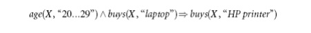
repeated predicates, which contain multiple occurrences of some predicates.
These rules are called hybrid-dimensional association rules. An example of such
a rule is the following, where the predicate buys is repeated:
Note that
database attributes can be categorical or quantitative. Categorical attributes
have a finite number of possible values, with no ordering among the values
(e.g., occupation, brand, color). Categorical attributes are also
called nominal attributes, because their values are ―names of things.‖ Quantitative attributes are
numeric and have an implicit ordering among values (e.g., age, income, price). Techniques for mining
multidimensional association rules can be categorized into two basic approaches regarding the treatment of quantitative
attributes.
Mining Multidimensional
Association Rules Using Static Discretization of Quantitative
Attributes
Quantitative
attributes, in this case, are discretized before mining using predefined
concept hierarchies or data discretization techniques, where numeric values are
replaced by interval labels. Categorical attributes may also be generalized to
higher conceptual levels if desired. If the resulting task-relevant data are
stored in a relational table, then any of the frequent itemset mining
algorithms we have discussed can be modified easily so as to find all frequent
predicate sets rather than frequent itemsets. In particular, instead of
searching on only one attribute like buys,
we need to search through all of the relevant attributes, treating each
attribute-value pair as an itemset.
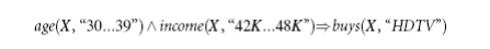
Mining Quantitative Association
Rules
Quantitative
association rules are multidimensional association rules in which the numeric
attributes are dynamically
discretized during the mining process so as to satisfy some mining criteria,
such as maximizing the confidence or compactness of the rules mined. In this
section, we focus specifically on how to mine quantitative association rules
having two quantitative attributes on the left-hand side of the rule and one
categorical attribute on the right-hand side of the rule. That is,

where Aquan1 and Aquan2 are tests on quantitative attribute intervals (where the
intervals are dynamically determined), and Acat
tests a categorical attribute from the task-relevant data. Such rules have been
referred to as two-dimensional quantitative association rules, because they
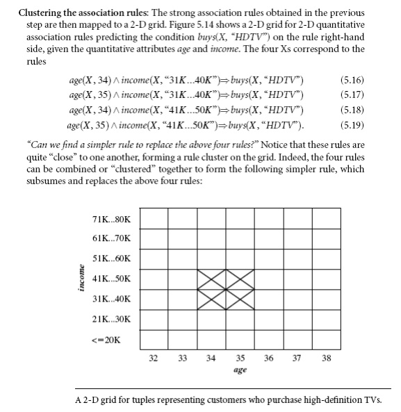
contain two quantitative dimensions. For instance, suppose you are curious
about the association relationship between pairs of quantitative attributes,
like customer age and income, and the type of television (such as high-definition TV, i.e., HDTV) that customers like to buy. An example
of such a 2-D quantitative association rule is
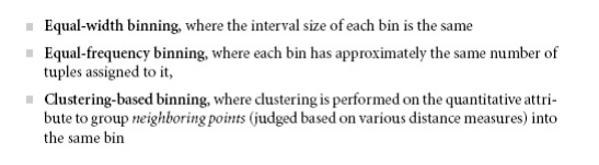
Binning: Quantitative
attributes can have a very wide range of values defining their domain. Just think about how big a 2-D grid would
be if we plotted age and income as axes, where each possible
value of age was assigned a unique
position on one axis, and similarly, each possible value of income was assigned a unique position on
the other axis! To keep grids down to a manageable size, we instead partition the ranges of quantitative attributes into
intervals. These intervals are dynamic in that they may later be further
combined during the mining process. The partitioning process is referred to as
binning, that is, where the intervals are considered ―bins.‖ Three common
binning strategies area as follows:
Finding frequent predicate sets: Once the
2-D array containing the count distribution for each category is set up, it can be scanned to find the frequent
predicate sets (those satisfying minimum support) that also satisfy minimum
confidence. Strong association rules can then be generated from these predicate
sets, using a rule generation algorithm.
Related Topics