Classification by Decision Tree Induction

Classification by Decision Tree Induction

Decision tree

^o     A flow-chart-like tree structure

^o     Internal node denotes a test on an attribute node (nonleaf node) denotes a test on an attribute

^o     Branch represents an outcome of the test

^o     Leaf nodes represent class labels or class distribution(Terminal node)

^o     The topmost node in a tree is the root node.

Decision tree generation consists of two phases

^o     Tree construction

^o     At start, all the training examples are at the root

^o     Partition examples recursively based on selected attributes ^Ø Tree pruning

^o     Identify and remove branches that reflect noise or outliers

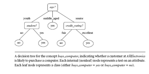
A typical decision tree is shown in Figure. It represents the concept buys computer, that is, it predicts whether a customer at AllElectronics is likely to purchase a computer. Internal nodes are denoted by rectangles, and leaf nodes are denoted by ovals. Some decision tree algorithms produce only binary trees (where each internal node branches to exactly two other nodes), whereas others can produce non binary trees.

“How are decision trees used for classification?” Given a tuple, X, for which the associated class label is unknown, the attribute values of the tuple are tested against the decision tree. A path is traced from the root to a leaf node, which holds the class prediction for that tuple. Decision trees can easily be converted to classification rules.

Decision Tree Induction

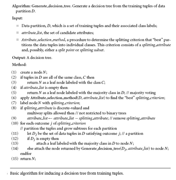
The tree starts as a single node, N, representing the training tuples in D (step 1)

If the tuples in D are all of the same class, then node N becomes a leaf and is labeled with that class (steps 2 and 3). Note that steps 4 and 5 are terminating conditions. All of the terminating conditions are explained at the end of the algorithm.

Otherwise, the algorithm calls Attribute selection method to determine the splitting criterion. The splitting criterion tells us which attribute to test at node N by determining the ―best‖ way to separate or partition the tuples in D into individual classes(step 6). The splitting criterion also tells us which branches to grow from node N with respect to the outcomes of the chosen test. More specifically, the splitting criterion indicates the splitting attribute and may also indicate either a split-point or a splitting subset. The splitting criterion is determined so that, ideally, the resulting partitions at each branch are as ―pure‖ as possible.

A partition is pure if all of the tuples in it belong to the same class. In other words, if we were to split up the tuples in D according to the mutually exclusive outcomes of the splitting criterion, we hope for the resulting partitions to be as pure as possible.

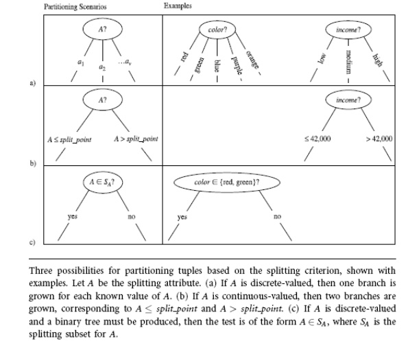
The node N is labeled with the splitting criterion, which serves as a test at the node (step 7). A branch is grown from node N for each of the outcomes of the splitting criterion. The tuples in D are partitioned accordingly (steps 10 to 11). There are three possible scenarios, as illustrated in Figure. Let A be the splitting attribute. A has v distinct values, {a1, a2, : : : , av}, based on the training data.

Attribute Selection Measures

An attribute selection measure is a heuristic for selecting the splitting criterion that ―best‖ separates a given data partition, D, of class-labeled training tuples into individual classes. If we were to split D into smaller partitions according to the outcomes of the splitting criterion, If the splitting attribute is continuous-valued or if we are restricted to binary trees then, respectively, either a split point or a splitting subset must also be determined as part of the splitting criterion This section describes three popular attribute selection measures—information gain, gain ratio, and gini inde

Information gain:ID3 uses information gain as its attribute selection measure.

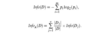
Information gain is defined as the difference between the original information requirement (i.e., based on just the proportion of classes) and the new requirement (i.e., obtained after partitioning on A). That is,

In other words, Gain(A) tells us how much would be gained by branching on A. It is the expected reduction in the information requirement caused by knowing the value of A. The attribute A with the highest information gain, (Gain(A)), is chosen as the splitting attribute at node N.

Example Induction of a decision tree using information gain.

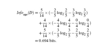
Table 6.1 presents a training set, D, of class-labeled tuples randomly selected from the AllElectronics customer database. (The data are adapted from [Qui86]. In this example, each attribute is discrete-valued. Continuous-valued attributes have been generalized.) The class label attribute, buys computer, has two distinct values (namely, {yes, no}); therefore, there are two distinct classes (that is, m = 2). Let class C1 correspond to yes and class C2 correspond to no. There are nine tuples of class yes and five tuples of class no. A (root) node N is created for the tuples in D. 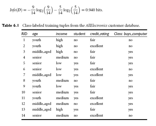To find the splitting criterion for these tuples, we must compute the information gain of each attribute. We first use Equation (6.1) to compute the expected information needed to classify a tuple in D:

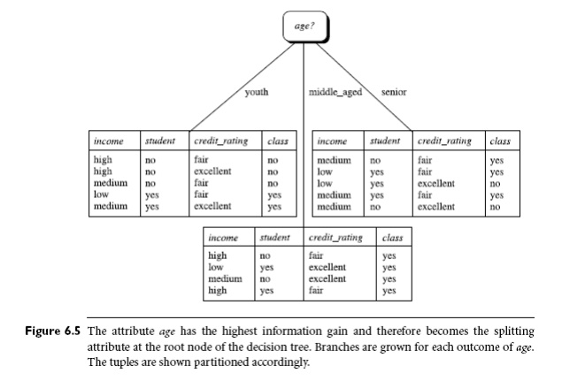
The expected information needed to classify a tuple in D if the tuples are partitioned according to age is

Hence, the gain in information from such a partitioning would be

Similarly, we can compute Gain(income) = 0.029 bits, Gain(student) = 0.151 bits, and Gain(credit rating) = 0.048 bits. Because age has the highest information gain among the attributes, it is selected as the splitting attribute. Node N is labeled with age, and branches are grown for each of the attribute’s values. The tuples are then partitioned accordingly, as shown in Figure 6.5. Notice that the tuples falling into the partition for age = middle aged all belong to the same class. Because they all belong to class “yes,” a leaf should therefore be created at the end of this branch and labeled with “yes.” The final decision tree returned by the algorithm is shown in Figure 6.5.