Advanced data analysis tools - Spreadsheet

Advanced data analysis tools

A spreadsheet is a “Flat file database”. Thus, database operations such as sorting, filtering can be done on spreadsheet. The “Data” menu of OpenOffice calc provides maximum data analysis tools such as sorting, filtering, validity etc., In this part, the sorting and filtering feature is to be learnt.

 

1. Database

 

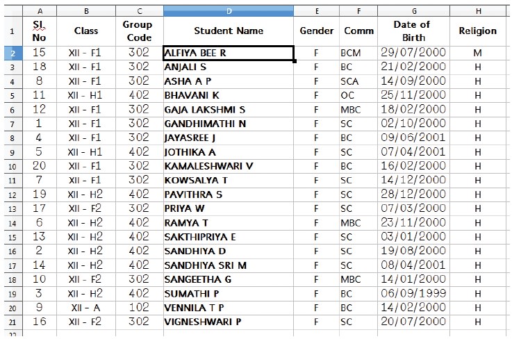
A database is a repository of collections of related data or facts. It arranges them in a specific structure. The table given below contains details of students in a class.

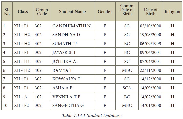
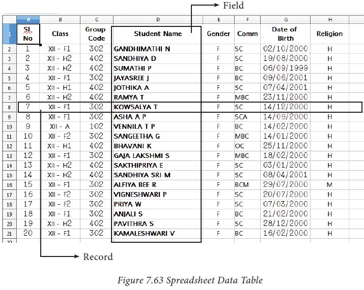
The entire collection or related data in one table is referred to as a File or a Table. Each row in a table represents a Record, which is a set of data for each database entry. Each table column represents a Field, which groups each piece or item of data among the records into specific categories. (Refer Figure 7.63)

 

2. Sorting:

 

Sorting is the process of arranging data in ascending or descending order. There are two types of sorting in OpenOffice Calc. They are,

 

i.    Simple Sorting

 

ii.   Multi Sorting

 

iii.  Sort by selection

 

(1) Simple Sorting

 

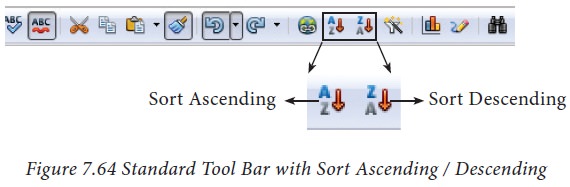
Arranging data using single column is known as simple sorting. For sorting the data, calc provide two icons on the standard tool bar viz. (1) Sort Ascending (2) Sort Descending.

 

·           Sort Ascending – Arrange data in alphabetical order (A to Z / Small to Large)

 

·           Sort Descending – Arrange data in reverse order (Z to A / Large to Small)

 

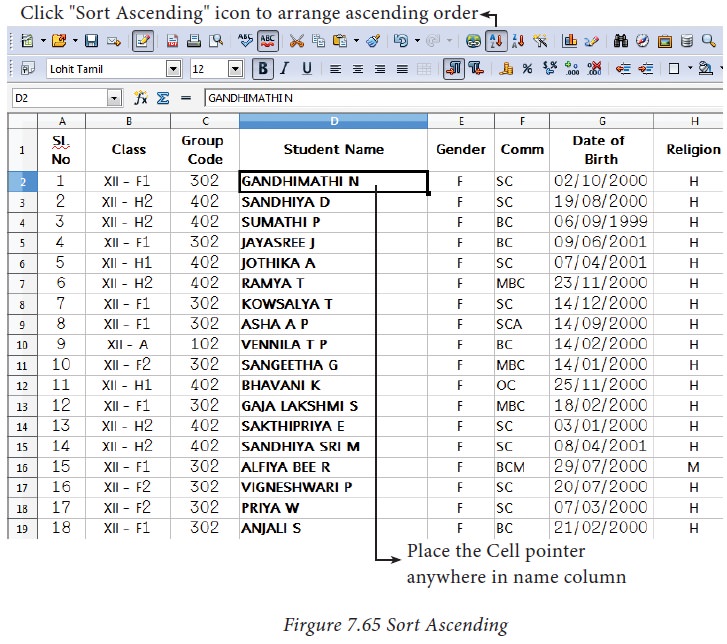
Sorting data

 

Step 1: Place cell pointer in the field (column) to be sorted

 

Step 2: Click Sort Ascending or Sort Descending icon

 

OpenOffice Calc, sort the data of selected column and its corresponding values present in other columns are also arranged simultaneously. Refer Figure 7.65

 

(2) Multi Sorting

 

Sorting data based on more than one field (column) is known as multi sorting. For example, the worksheet containing data of 20 students belongs to different groups and classes. To rearrange this data alphabetically by name and group code, multi sorting is used. Refer Figure 7.66.

 

Multi-sorting data

 

Step 1: Select Data -> Sort

 

Name are arranged in Ascending order According to names, other data also rearranged

 

Step 2:  Sort dialog box appears. (Refer Figure 7.67)

 

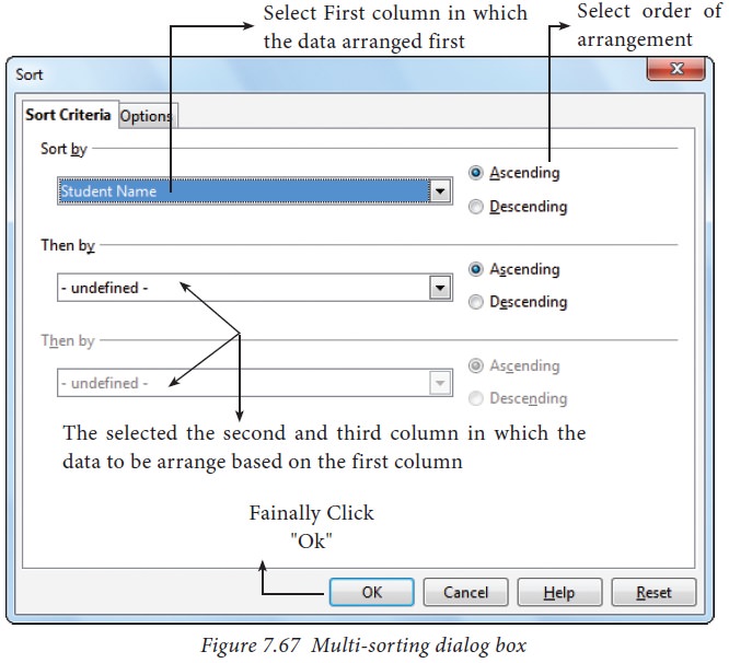
Step 3:  Select the field name (Student name) in which you want to sort from the “sort by” dropdown list box and then choose order of sorting i.e. Ascending or Descending. Ascending is the default selection.

 

Step 4:  Select another field name (Group Code) from the “Then by” dropdown list box and choose the order of sorting to this column.

 

Step 5:  Click “OK” button.

 

In OpenOffice Calc, multi sort can be done only for three fields.

(3) Sort by selection

 

In Calc sorting can be done on selected range. But this kind of sorting is generally not recommended, because the other relevant data are also not sorted. Therefore, OpenOffice Calc displays a warnning message for this type of sorting. Refer Figure 7.68.

 

Sorting data by selection:

 

Step 1:  Select any particular field in which you want sort.

 

Step 2:  Click required Sort icon from standard tool bar or Data -> Sort command.

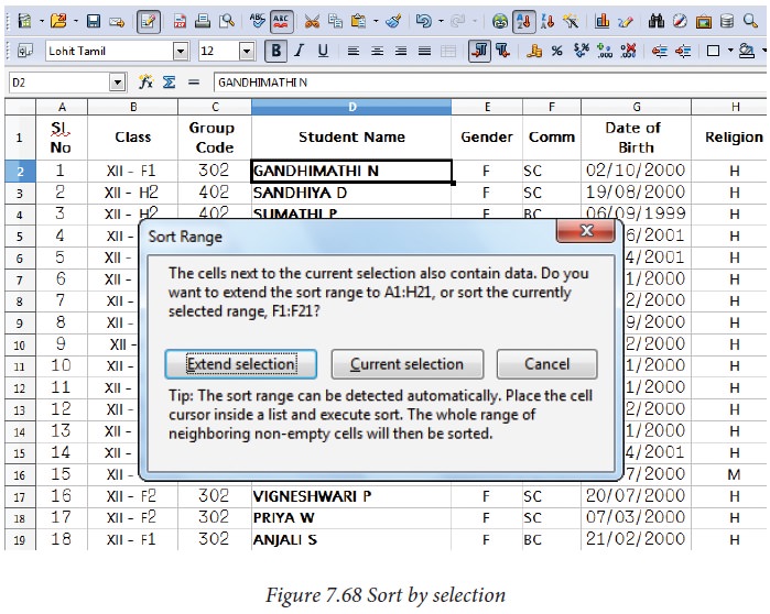
Calc, display a “Sort Range” warning message as shown in the Figure 7.68

“Sort Range” message box has two options, viz. (1) Extend selection (2) Current selection.

 

Step 3:  “Extend Selection” – Sort all the data based on the selection.

“Current Selection” – Sort only the selected range of data, remaining data are not sorted.

 

3. Filtering

 

Filter is a way of limiting the information that appears on screen. 

Filters are a feature for displaying and browsing a selected list or subset of data from a worksheet. The visible records satisfy the condition that the user sets. Those that do not satisfy the condition are only hidden, but not removed.

 

OpenOffice Calc allows three types of filters. They are AutoFilter, Standard Filter and Advanced Filter.

 

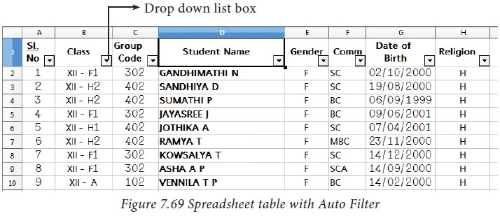
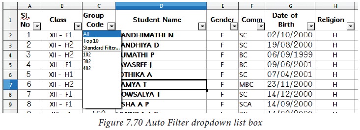
(1) Auto Filter:

 

Auto Filter applies a drop-down list box to each field (columns) filled with similar data available in that field. Using the list box item, you can filter the data that matches the criteria of the data concerned.

 

Using Auto Filter:

 

·          Click Auto Filter icon  available on the “Standard tools bar” (or) Click Data -> Filter ->  Auto Filter

 

·           The list box contains similar data in the fields. Refer Figure 7.69 and 7.70

 

·           Each list box item will be considered as filter criteria.

·           Select the data item from the list box. Now, Calc shows only the records which are satisfy the selected criteria.

 

Example:

 

If you want to apply an auto filter to the contents of the table 7.14.1, follow the following two steps

 

Step 1: Place cell pointer anywhere in the table

 

Step 2: Click Auto Filter icon   available on the “Standard tools bar” (or) Click Data - > Filter -> Auto Filter

 

In the above table, if you want to view only the students belongs to the Group code 402;

 

•     Click the dropdown list box’s drop arrow (a tiny triangle) to get the filter criteria. (Refer Figure 7.70)

 

•     Select group code 402 from the list

 

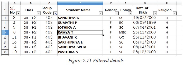
•     The spreadsheet displays only the student’s details those who are studing in group code 402 (Refer Figure 7.71) and the remaining details are only hidden.

 

Removing Auto Filter:

 

•     To remove auto filter, click “Auto filter” icon once again .

 

•     The original table is displayed without filter.

 

(2) Standard Filter: Auto filter is used only for single criteria on a data, whereas the Standard filter is used for multiple critieria to filter.

 

Step 1:

 

·           Select Data ->  Filter -> Standard Filter.

 

 

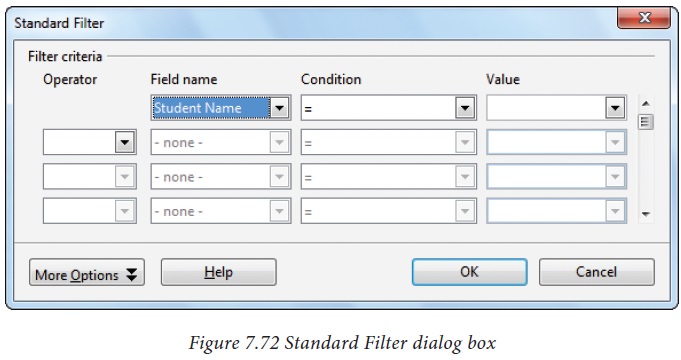
·           Now, the entire data is selected and "Standard Filter" dialog box dispalys as shown in Figure 7.73.

 

Step 2:

 

·           Select the column heading from the “Filed name” list box for first criteria.

 

·           Select conditional opeator such as >, <, = etc., from “Condition” list box.

 

·           Type or select the value of critera in the “Value” box.

 

Step 3:

 

·           Select the one of the logical operator (And / Or) from “Operator” list box to fix second criteria.

 

·           Follow the step 2, for the next criteria.

 

Step 4:

 

Click “OK” to finish.

 

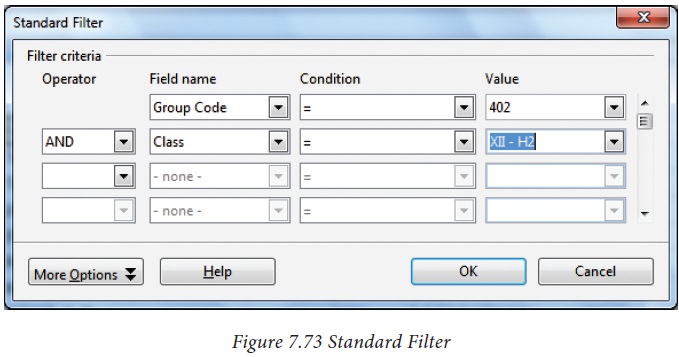
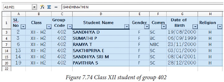
Example for Standard filter:

If you want to filter the records of “BC” students of group code 402 from the table 7.14.1

 

Step 1: Select Data oFilter -> Standard Filter

• Now, “Standard Filter” dialog box appears as in Figure 7.73

 

Step 2: In “Standard Filter” dialog box, select the first criteria;

• Select Field name as Group code

• Select Condition as =

• Type or select Value as 402

 

Step 3: To select the second criteria;

• Select Operator as “AND”

• Select Field name as Class

• Select Condition as =

• Type or select Value as XII- H2

 

Step 4: Click “OK”

 

·           Now, the table displays only the recods which are match for the given two criteria. Refer Figure 7.74.

 

Remove Standard Filter:

 

Select Data -> Filter -> Remove Filter

·           “Header” tab is used to create header

·           “Footer” tab is used to create footer