Using Heuristics in Query Optimization

Using Heuristics in Query Optimization

In this section we discuss optimization techniques that apply heuristic rules to modify the internal representation of a query—which is usually in the form of a query tree or a query graph data structure—to improve its expected performance. The scanner and parser of an SQL query first generate a data structure that corresponds to an initial query representation, which is then optimized according to heuristic rules. This leads to an optimized query representation, which corresponds to the query execution strategy. Following that, a query execution plan is generated to execute groups of operations based on the access paths available on the files involved in the query.

One of the main heuristic rules is to apply SELECT and PROJECT operations before applying the JOIN or other binary operations, because the size of the file resulting from a binary operation—such as JOIN—is usually a multiplicative function of the sizes of the input files. The SELECT and PROJECT operations reduce the size of a file and hence should be applied before a join or other binary operation.

In Section 19.7.1 we reiterate the query tree and query graph notations that we introduced earlier in the context of relational algebra and calculus in Sections 6.3.5 and 6.6.5, respectively. These can be used as the basis for the data structures that are used for internal representation of queries. A query tree is used to represent a relational algebra or extended relational algebra expression, whereas a query graph is used to represent a relational calculus expression. Then in Section 19.7.2 we show how heuristic optimization rules are applied to convert an initial query tree into an equivalent query tree, which represents a different relational algebra expression that is more efficient to execute but gives the same result as the original tree. We also discuss the equivalence of various relational algebra expressions. Finally, Section 19.7.3 discusses the generation of query execution plans.

1. Notation for Query Trees and Query Graphs

A query tree is a tree data structure that corresponds to a relational algebra expression. It represents the input relations of the query as leaf nodes of the tree, and rep-resents the relational algebra operations as internal nodes. An execution of the query tree consists of executing an internal node operation whenever its operands are available and then replacing that internal node by the relation that results from executing the operation. The order of execution of operations starts at the leaf nodes, which represents the input database relations for the query, and ends at the root node, which represents the final operation of the query. The execution terminates when the root node operation is executed and produces the result relation for the query.

Figure 19.4a shows a query tree (the same as shown in Figure 6.9) for query Q2 in Chapters 4 to 6: For every project located in ‘Stafford’, retrieve the project number, the controlling department number, and the department manager’s last name, address, and birthdate. This query is specified on the COMPANY relational schema in Figure 3.5 and corresponds to the following relational algebra expression:

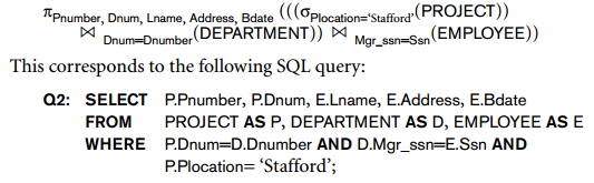
In Figure 19.4a, the leaf nodes P, D, and E represent the three relations PROJECT, DEPARTMENT, and EMPLOYEE, respectively, and the internal tree nodes represent the relational algebra operations of the expression. When this query tree is executed, the node marked (1) in Figure 19.4a must begin execution before node (2) because some resulting tuples of operation (1) must be available before we can begin executing operation (2). Similarly, node (2) must begin executing and producing results before node (3) can start execution, and so on.

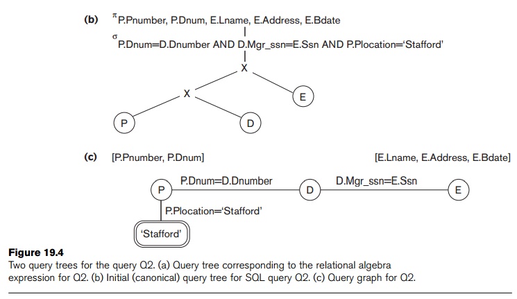
As we can see, the query tree represents a specific order of operations for executing a query. A more neutral data structure for representation of a query is the query graph notation. Figure 19.4c (the same as shown in Figure 6.13) shows the query graph for query Q2. Relations in the query are represented by relation nodes, which are displayed as single circles. Constant values, typically from the query selection conditions, are represented by constant nodes, which are displayed as double circles or ovals. Selection and join conditions are represented by the graph edges, as shown in Figure 19.4c. Finally, the attributes to be retrieved from each relation are dis-played in square brackets above each relation.

The query graph representation does not indicate an order on which operations to perform first. There is only a single graph corresponding to each query. Although some optimization techniques were based on query graphs, it is now generally accepted that query trees are preferable because, in practice, the query optimizer needs to show the order of operations for query execution, which is not possible in query graphs.

2. Heuristic Optimization of Query Trees

In general, many different relational algebra expressions—and hence many different query trees—can be equivalent; that is, they can represent the same query.

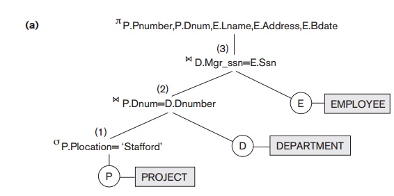
The query parser will typically generate a standard initial query tree to correspond to an SQL query, without doing any optimization. For example, for a SELECT-PROJECT-JOIN query, such as Q2, the initial tree is shown in Figure 19.4(b). The CARTESIAN PRODUCT of the relations specified in the FROM clause is first applied; then the selection and join conditions of the WHERE clause are applied, followed by the projection on the SELECT clause attributes. Such a canonical query tree represents a relational algebra expression that is very inefficient if executed directly, because of the CARTESIAN PRODUCT (×) operations. For example, if the PROJECT, DEPARTMENT, and EMPLOYEE relations had record sizes of 100, 50, and 150 bytes and contained 100, 20, and 5,000 tuples, respectively, the result of the CARTESIAN PRODUCT would contain 10 million tuples of record size 300 bytes each. However, the initial query tree in Figure 19.4(b) is in a simple standard form that can be eas-ily created from the SQL query. It will never be executed. The heuristic query optimizer will transform this initial query tree into an equivalent final query tree that is efficient to execute.

The optimizer must include rules for equivalence among relational algebra expressions that can be applied to transform the initial tree into the final, optimized query tree. First we discuss informally how a query tree is transformed by using heuristics, and then we discuss general transformation rules and show how they can be used in an algebraic heuristic optimizer.

Example of Transforming a Query. Consider the following query Q on the data-base in Figure 3.5: Find the last names of employees born after 1957 who work on a project named ‘Aquarius’. This query can be specified in SQL as follows:

        SELECT  Lname

FROMEMPLOYEE, WORKS_ON, PROJECT

WHERE  Pname=‘Aquarius’ AND Pnumber=Pno AND Essn=Ssn

AND Bdate > ‘1957-12-31’;

The initial query tree for Q is shown in Figure 19.5(a). Executing this tree directly first creates a very large file containing the CARTESIAN PRODUCT of the entire EMPLOYEE, WORKS_ON, and PROJECT files. That is why the initial query tree is never executed, but is transformed into another equivalent tree that is efficient to

Figure 19.5

Steps in converting a query tree during heuristic optimization.

      Initial (canonical) query tree for SQL query Q.

      Moving SELECT operations down the query tree.

      Applying the more restrictive SELECT operation first.

      Replacing CARTESIAN PRODUCT and SELECT with JOIN operations.

Moving PROJECT operations down the query tree.

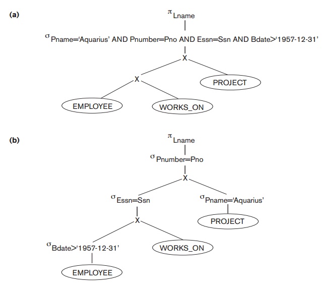
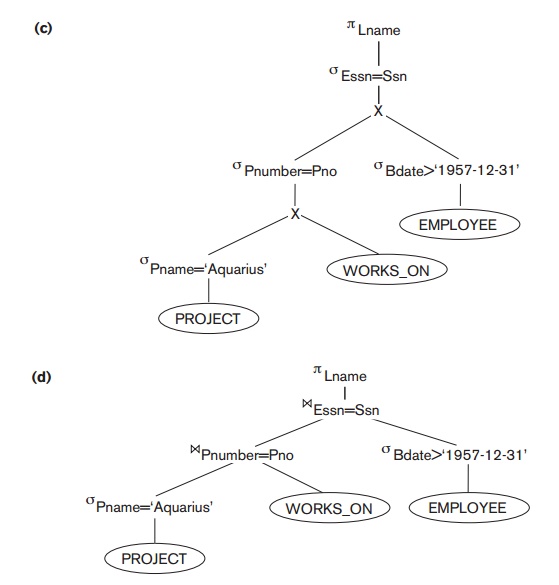
execute. This particular query needs only one record from the PROJECT relation— for the ‘Aquarius’ project—and only the EMPLOYEE records for those whose date of birth is after ‘1957-12-31’. Figure 19.5(b) shows an improved query tree that first applies the SELECT operations to reduce the number of tuples that appear in the CARTESIAN PRODUCT.

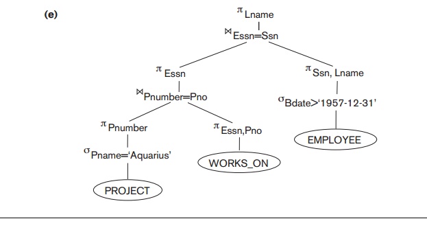
A further improvement is achieved by switching the positions of the EMPLOYEE and PROJECT relations in the tree, as shown in Figure 19.5(c). This uses the information that Pnumber is a key attribute of the PROJECT relation, and hence the SELECT operation on the PROJECT relation will retrieve a single record only. We can further improve the query tree by replacing any CARTESIAN PRODUCT operation that is followed by a join condition with a JOIN operation, as shown in Figure 19.5(d). Another improvement is to keep only the attributes needed by subsequent operations in the intermediate relations, by including PROJECT (π) operations as early as possible in the query tree, as shown in Figure 19.5(e). This reduces the attributes (columns) of the intermediate relations, whereas the SELECT operations reduce the number of tuples (records).

As the preceding example demonstrates, a query tree can be transformed step by step into an equivalent query tree that is more efficient to execute. However, we must make sure that the transformation steps always lead to an equivalent query tree. To do this, the query optimizer must know which transformation rules preserve this equivalence. We discuss some of these transformation rules next.

General Transformation Rules for Relational Algebra Operations. There are many rules for transforming relational algebra operations into equivalent ones. For query optimization purposes, we are interested in the meaning of the operations and the resulting relations. Hence, if two relations have the same set of attributes in a different order but the two relations represent the same information, we consider the relations to be equivalent. In Section 3.1.2 we gave an alternative definition of relation that makes the order of attributes unimportant; we will use this definition here. We will state some transformation rules that are useful in query optimization, without proving them:

        Cascade of σ A conjunctive selection condition can be broken up into a cascade (that is, a sequence) of individual σ operations:

^σc₁ AND c₂ AND . . . AND c_n^(R)   ≡ ^σc₁ ^(σc₂ ^(...(σc_n^(R))...))

        Commutativity of σ. The σ operation is commutative: σ_c1 (σ_c2(R)) === σ_c2 (σ_c1(R))

        Cascade of π. In a cascade (sequence) of π operations, all but the last one can be ignored:

^πList₁ ^(πList₂ ^(...(πList_n^(R))...))≡^πList₁^(R)

        Commuting σ with π. If the selection condition c involves only those attributes A₁, . . . , A_n in the projection list, the two operations can be commuted:

        ^πA₁, A₂, ..., A_n ^(σc ^(R))≡^σc ^(πA₁, A₂, ..., A_n ^(R))

       Commutativity of >< (and ×). The join operation is commutative, as is the × operation:

            >< _c S ≡ S >< _c R

            × S ≡ S × R

Notice that although the order of attributes may not be the same in the relations resulting from the two joins (or two Cartesian products), the meaning is the same because the order of attributes is not important in the alternative definition of relation.

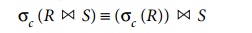
       Commuting σ with >< (or ×). If all the attributes in the selection condition c involve only the attributes of one of the relations being joined—say, R—the two operations can be commuted as follows:

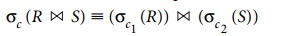
Alternatively, if the selection condition c can be written as (c₁ AND c₂), where condition c₁ involves only the attributes of R and condition c₂ involves only the attributes of S, the operations commute as follows:

The same rules apply if the >< is replaced by a × operation.

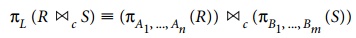
       Commuting π with >< (or ×). Suppose that the projection list is L = {A₁, ..., A_n, B₁, ..., B_m} , where A₁, ..., A_n are attributes of R and B₁, ..., B_m are attributes of S. If the join condition c involves only attributes in L, the two operations can be commuted as follows:

If the join condition c contains additional attributes not in L, these must be added to the projection list, and a final π operation is needed. For example, if attributes A_n+1, ..., A_n+k of R and B_m+1, ..., B_m+p of S are involved in the join condition c but are not in the projection list L, the operations commute as follows:

For x, there is no condition c, so the first transformation rule always applies by replacing >< _c with ×.

       Commutativity of set operations. The set operations ∪ and ∩ are commutative but − is not.

       Associativity of  >< , ×, ∪, and ∩. These four operations are individually associative; that is, if θ stands for any one of these four operations (through-out the expression), we have:

(R θ S) θ T ≡ R θ (S θ T)

       Commuting σ with set operations. The σ operation commutes with ∪, ∩, and −. If θ stands for any one of these three operations (throughout the expression), we have:

σ_c (R θ S) ≡ (σ_c (R)) θ (σ_c (S))

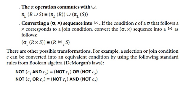
Additional transformations discussed in Chapters 4, 5, and 6 are not repeated here. We discuss next how transformations can be used in heuristic optimization.

Outline of a Heuristic Algebraic Optimization Algorithm. We can now out-line the steps of an algorithm that utilizes some of the above rules to transform an initial query tree into a final tree that is more efficient to execute (in most cases). The algorithm will lead to transformations similar to those discussed in our example in Figure 19.5. The steps of the algorithm are as follows:

1.   Using Rule 1, break up any SELECT operations with conjunctive conditions into a cascade of SELECT operations. This permits a greater degree of freedom in moving SELECT operations down different branches of the tree.

2.   Using Rules 2, 4, 6, and 10 concerning the commutativity of SELECT with other operations, move each SELECT operation as far down the query tree as is permitted by the attributes involved in the select condition. If the condition involves attributes from only one table, which means that it represents a selection condition, the operation is moved all the way to the leaf node that represents this table. If the condition involves attributes from two tables, which means that it represents a join condition, the condition is moved to a location down the tree after the two tables are combined.

^3.        Using Rules 5 and 9 concerning commutativity and associativity of binary operations, rearrange the leaf nodes of the tree using the following criteria. First, position the leaf node relations with the most restrictive SELECT operations so they are executed first in the query tree representation. The definition of most restrictive SELECT can mean either the ones that produce a relation with the fewest tuples or with the smallest absolute size.¹⁷ Another possibility is to define the most restrictive SELECT as the one with the small-est selectivity; this is more practical because estimates of selectivities are often available in the DBMS catalog. Second, make sure that the ordering of leaf nodes does not cause CARTESIAN PRODUCT operations; for example, if the two relations with the most restrictive SELECT do not have a direct join condition between them, it may be desirable to change the order of leaf nodes to avoid Cartesian products.

4.   Using Rule 12, combine a CARTESIAN PRODUCT operation with a subsequent SELECT operation in the tree into a JOIN operation, if the condition represents a join condition.

5.   Using Rules 3, 4, 7, and 11 concerning the cascading of PROJECT and the commuting of PROJECT with other operations, break down and move lists of projection attributes down the tree as far as possible by creating new PROJECT operations as needed. Only those attributes needed in the query result and in subsequent operations in the query tree should be kept after each PROJECT operation.

6.   Identify subtrees that represent groups of operations that can be executed by a single algorithm.

In our example, Figure 19.5(b) shows the tree in Figure 19.5(a) after applying steps 1 and 2 of the algorithm; Figure 19.5(c) shows the tree after step 3; Figure 19.5(d) after step 4; and Figure 19.5(e) after step 5. In step 6 we may group together the operations in the subtree whose root is the operation π_{Essn i}nto a single algorithm. We may also group the remaining operations into another subtree, where the tuples resulting from the first algorithm replace the subtree whose root is the operation π_Essn, because the first grouping means that this subtree is executed first.

Summary of Heuristics for Algebraic Optimization. The main heuristic is to apply first the operations that reduce the size of intermediate results. This includes performing as early as possible SELECT operations to reduce the number of tuples and PROJECT operations to reduce the number of attributes—by moving SELECT and PROJECT operations as far down the tree as possible. Additionally, the SELECT and JOIN operations that are most restrictive—that is, result in relations with the fewest tuples or with the smallest absolute size—should be executed before other similar operations. The latter rule is accomplished through reordering the leaf nodes of the tree among themselves while avoiding Cartesian products, and adjusting the rest of the tree appropriately.

3. Converting Query Trees into Query Execution Plans

An execution plan for a relational algebra expression represented as a query tree includes information about the access methods available for each relation as well as the algorithms to be used in computing the relational operators represented in the tree. As a simple example, consider query Q1 from Chapter 4, whose corresponding relational algebra expression is

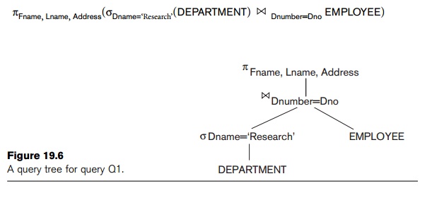
The query tree is shown in Figure 19.6. To convert this into an execution plan, the optimizer might choose an index search for the SELECT operation on DEPARTMENT (assuming one exists), a single-loop join algorithm that loops over the records in the result of the SELECT operation on DEPARTMENT for the join operation (assuming an index exists on the Dno attribute of EMPLOYEE), and a scan of the JOIN result for input to the PROJECT operator. Additionally, the approach taken for executing the query may specify a materialized or a pipelined evaluation, although in general a pipelined evaluation is preferred whenever feasible.

With materialized evaluation, the result of an operation is stored as a temporary relation (that is, the result is physically materialized). For instance, the JOIN operation can be computed and the entire result stored as a temporary relation, which is then read as input by the algorithm that computes the PROJECT operation, which would produce the query result table. On the other hand, with pipelined evaluation, as the resulting tuples of an operation are produced, they are forwarded directly to the next operation in the query sequence. For example, as the selected tuples from DEPARTMENT are produced by the SELECT operation, they are placed in a buffer; the JOIN operation algorithm would then consume the tuples from the buffer, and those tuples that result from the JOIN operation are pipelined to the projection operation algorithm. The advantage of pipelining is the cost savings in not having to write the intermediate results to disk and not having to read them back for the next operation.