Example to Illustrate Cost-Based Query Optimization

Example to Illustrate Cost-Based Query Optimization

We will consider query Q2 and its query tree shown in Figure 19.4(a) to illustrate cost-based query optimization:

Q2:      SELECT Pnumber, Dnum, Lname, Address, Bdate

FROM               PROJECT, DEPARTMENT, EMPLOYEE

WHERE             Dnum=Dnumber AND Mgr_ssn=Ssn AND

Plocation=‘Stafford’;

Suppose we have the information about the relations shown in Figure 19.8. The LOW_VALUE and HIGH_VALUE statistics have been normalized for clarity. The tree in Figure 19.4(a) is assumed to represent the result of the algebraic heuristic opti-mization process and the start of cost-based optimization (in this example, we assume that the heuristic optimizer does not push the projection operations down the tree).

The first cost-based optimization to consider is join ordering. As previously men-tioned, we assume the optimizer considers only left-deep trees, so the potential join orders—without CARTESIAN PRODUCT—are:

Assume that the selection operation has already been applied to the PROJECT rela-tion. If we assume a materialized approach, then a new temporary relation is created after each join operation. To examine the cost of join order (1), the first join is between PROJECT and DEPARTMENT. Both the join method and the access methods for the input relations must be determined. Since DEPARTMENT has no index according to Figure 19.8, the only available access method is a table scan (that is, a linear search). The PROJECT relation will have the selection operation performed before the join, so two options exist: table scan (linear search) or utiliz-ing its PROJ_PLOC index, so the optimizer must compare their estimated costs.

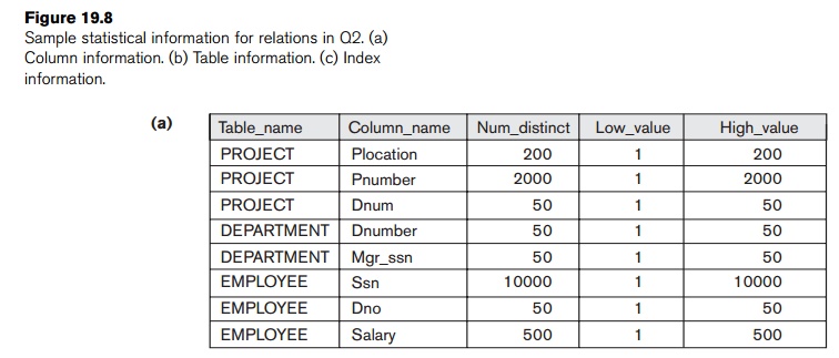
The statistical information on the PROJ_PLOC index (see Figure 19.8) shows the number of index levels x = 2 (root plus leaf levels). The index is nonunique (because Plocation is not a key of PROJECT), so the optimizer assumes a uniform data distribution and estimates the number of record pointers for each Plocation value to be 10. This is computed from the tables in Figure 19.8 by multiplying

Selectivity _* Num_rows, where Selectivity is estimated by 1/Num_distinct. So the cost of using the index and accessing the records is estimated to be 12 block accesses (2 for the index and 10 for the data blocks). The cost of a table scan is estimated to be 100 block accesses, so the index access is more efficient as expected.

In the materialized approach, a temporary file TEMP1 of size 1 block is created to hold the result of the selection operation. The file size is calculated by determining the blocking factor using the formula Num_rows/Blocks, which gives 2000/100 or 20 rows per block. Hence, the 10 records selected from the PROJECT relation will fit into a single block. Now we can compute the estimated cost of the first join. We will consider only the nested-loop join method, where the outer relation is the tempo-rary file, TEMP1, and the inner relation is DEPARTMENT. Since the entire TEMP1 file fits in the available buffer space, we need to read each of the DEPARTMENT table’s five blocks only once, so the join cost is six block accesses plus the cost of writing the temporary result file, TEMP2. The optimizer would have to determine the size of TEMP2. Since the join attribute Dnumber is the key for DEPARTMENT, any Dnum value from TEMP1 will join with at most one record from DEPARTMENT, so the number of rows in TEMP2 will be equal to the number of rows in TEMP1, which is 10. The optimizer would determine the record size for TEMP2 and the number of blocks needed to store these 10 rows. For brevity, assume that the blocking factor for TEMP2 is five rows per block, so a total of two blocks are needed to store TEMP2.

Finally, the cost of the last join needs to be estimated. We can use a single-loop join on TEMP2 since in this case the index EMP_SSN (see Figure 19.8) can be used to probe and locate matching records from EMPLOYEE. Hence, the join method would involve reading in each block of TEMP2 and looking up each of the five Mgr_ssn val-ues using the EMP_SSN index. Each index lookup would require a root access, a leaf access, and a data block access (x+1, where the number of levels x is 2). So, 10 lookups require 30 block accesses. Adding the two block accesses for TEMP2 gives a total of 32 block accesses for this join.

For the final projection, assume pipelining is used to produce the final result, which does not require additional block accesses, so the total cost for join order (1) is esti-mated as the sum of the previous costs. The optimizer would then estimate costs in a similar manner for the other three join orders and choose the one with the lowest estimate. We leave this as an exercise for the reader.