Examples of Cost Functions for JOIN

Examples of Cost Functions for JOIN

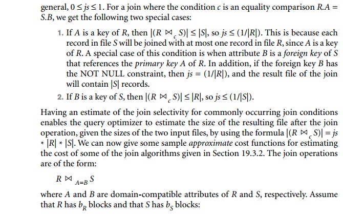
To develop reasonably accurate cost functions for JOIN operations, we need to have an estimate for the size (number of tuples) of the file that results after the JOIN operation. This is usually kept as a ratio of the size (number of tuples) of the resulting join file to the size of the CARTESIAN PRODUCT file, if both are applied to the same input files, and it is called the join selectivity ( js). If we denote the number of tuples of a relation R by |R|, we have:

If there is no join condition c, then js = 1 and the join is the same as the CARTESIAN PRODUCT. If no tuples from the relations satisfy the join condition, then js = 0. In 

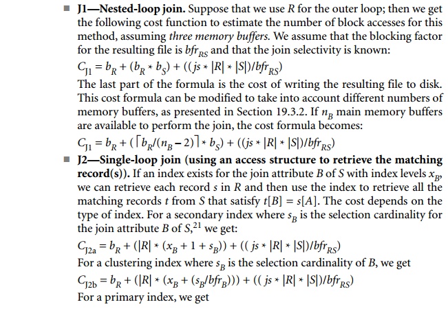
C_J2c = b_R + (|R| _* (x_B + 1)) + (( j s _* |R| _* |S|)/bfr_RS)

If a hash key exists for one of the two join attributes—say, B of S—we get

C_J2d = b_R + (|R| _* h) + (( j s _* |R| _* |S|)/bfr_RS)

where h ≥ 1 is the average number of block accesses to retrieve a record, given its hash key value. Usually, h is estimated to be 1 for static and linear hashing and 2 for extendible hashing.

        J3—Sort-merge join. If the files are already sorted on the join attributes, the

cost function for this method is

C_J3a = b_R + b_S + (( j s _* |R| _* |S|)/bfr_RS)

If we must sort the files, the cost of sorting must be added. We can use the formulas from Section 19.2 to estimate the sorting cost.

Example of Using the Cost Functions. Suppose that we have the EMPLOYEE file described in the example in the previous section, and assume that the DEPARTMENT file in Figure 3.5 consists of r_D = 125 records stored in b_D = 13 disk blocks. Consider the following two join operations:

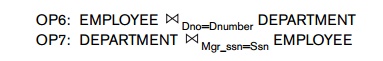
Suppose that we have a primary index on Dnumber of DEPARTMENT with x_Dnumber= 1 level and a secondary index on Mgr_ssn of DEPARTMENT with selection cardinality s_{Mgr_ssn}= 1 and levels x_{Mgr_ssn}= 2. Assume that the join selectivity for OP6 is js_OP6 = (1/|DEPARTMENT|) = 1/125 because Dnumber is a key of DEPARTMENT. Also assume that the blocking factor for the resulting join file is bfr_ED= 4 records per block. We can estimate the worst-case costs for the JOIN operation OP6 using the applicable methods J1 and J2 as follows:

1. Using method J1 with EMPLOYEE as outer loop:

^C_J1          ^{= b}_E ^{+ (b}_E * ^b_D^{) + (( js}_OP6 * ^r_E * ^r_D^)/bfr_ED⁾

            2000 + (2000 _* 13) + (((1/125) _* 10,000 _* 125)/4) = 30,500

        2. Using method J1 with DEPARTMENT as outer loop:

^C_J1          ^{= b}_D ^{+ (b}_E * ^b_D^{) + (( js}_OP6 * ^r_E * ^r_D)^/bfr_ED⁾

            13 + (13 _* 2000) + (((1/125) _* 10,000 _* 125/4) = 28,513

        3. Using method J2 with EMPLOYEE as outer loop:

^C_J2c  ^{= b}_E ^{+ (r}_E * ^(x_Dnumber^{+ 1)) + (( js}_OP6 * ^r_E * ^r_D^)/bfr_ED

            2000 + (10,000 _* 2) + (((1/125) _* 10,000 _* 125/4) = 24,500

        4. Using method J2 with DEPARTMENT as outer loop:

^C_J2a  ^{= b}_D ^{+ (r}_D * ^(x_Dno ^{+ s}_Dno^{)) + (( js}_OP6 * ^r_E * ^r_D^)/bfr_ED⁾

            13 + (125 _* (2 + 80)) + (((1/125) _* 10,000 _* 125/4) = 12,763

Case 4 has the lowest cost estimate and will be chosen. Notice that in case 2 above, if 15 memory buffers (or more) were available for executing the join instead of just 3, 13 of them could be used to hold the entire DEPARTMENT relation (outer loop relation) in memory, one could be used as buffer for the result, and one would be used to hold one block at a time of the EMPLOYEE file (inner loop file), and the cost

for case 2 could be drastically reduced to just b_E + b_D + (( js_{OP6 *} r_{E *} r_D)/bfr_ED) or 4,513, as discussed in Section 19.3.2. If some other number of main memory buffers was available, say n_B = 10, then the cost for case 2 would be calculated as follows, which would also give better performance than case 4:

C_J1  = b_D + (  b_D/(n_B – 2)       _* b_E) + ((js _* |R| _* |S|)/bfr_RS)

            =13 + (  13/8  _* 2000) + (((1/125) _* 10,000 _* 125/4) = 28,513

            =13 + (2 _* 2000) + 2500 = 6,513

As an exercise, the reader should perform a similar analysis for OP7.