Maximal flow model

MAXIMAL FLOW MODEL

Consider a network of pipelines that transports crude oil from oil wells to refineries. Intermediate booster and pumping stations are installed at appropriate design distances to move the crude in the network. Each pipe segment has a finite maximum discharge rate of crude flow (or capacity). A pipe segment may be uni- or bidirectional, depending on its design. Figure 6.27 demonstrates a typical pipeline network. How can we deter-mine the maximum capacity of the network between the wells and the refineries?

The solution of the proposed problem requires equipping the network with a single source and a single sink by using unidirectional infinite capacity arcs as shown by dashed arcs in Figure 6.27.

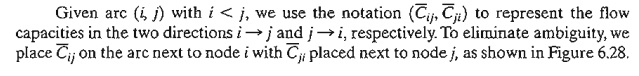
1. Enumeration of Cuts

A cut defines a set of arcs which when deleted from the network will cause a total disruption of flow between the source and sink nodes. The cut capacity equals the sum of the capacities of its arcs. Among all possible cuts in the network, the cut with the smallest capacity gives the maximum flow in the network.

Example 6.4-1

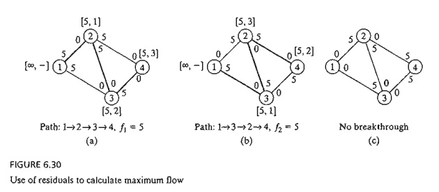
Consider the network in Figure 6.29. The bidirectional capacities are shown on the respective arcs using the convention in Figure 6.28. For example, for arc (3,4), the flow limit is 10 units from 3 to 4 and 5 units from 4 to 3.

Figure 6.29 illustrates three cuts whose capacities are computed in the following table.

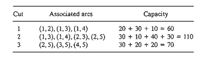
FIGURE 6.27

Capacitated network connecting wells and refineries through booster stations

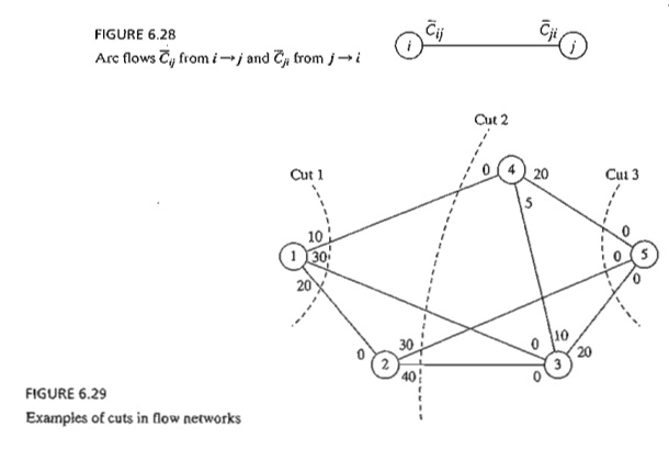
The only information we can glean from the three cuts is that the maximum flow in the net-work cannot exceed 60 units. To determine the maximum flow, it is necessary to enumerate all the cuts, a difficult task for the general network. Thus, the need for an efficient algorithm is imperative.

PROBLEM SET 6.4A

*1. For the network in Figure 6.29, determine two additional cuts, and find their capacities.

2. Maximal Flow Algorithm

The maximal flow algorithm is based on finding breakthrough paths with net positive flow between the source and sink nodes. Each path commits part or all of the capaci- ties of its arcs to the total flow in the network.

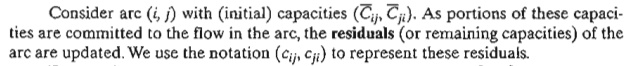
For a node j that receives flow from node i, we attach a label [a_i, i], where aj is the flow from node i to node j. The steps of the algorithm are thus summarized as follows.

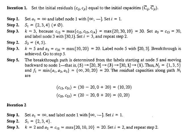
Set a_k = c_ik and label node k with [a_k i]. If k = n, the sink node has been labeled, and a breakthrough path. is found, go to step 5. Otherwise, set i = k, and go to step 2.

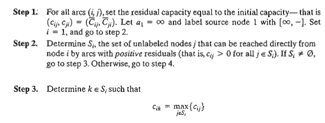
Step 4. (Backtracking). If i = 1, no breakthrough is possible; go to step 6. Otherwise, let r be the node that has been labeled immediately before current node i and remove i from the set of nodes adjacent to r. Set i = r, and go to step 2.

Step 5. (Determination ofresiduals). Let N_p = (1, k₁ k2, .. . , n) define the nodes of the pth breakthrough path from source node 1 to sink node n. Then the max-imum flow along the path is computed as

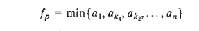
The residual capacity of each arc along the breakthrough path is decreased by f _p in the direction of the flow and increased by f _p in the reverse direction-that is, for nodes i and j on the path, the residual flow is changed from the current (Cij, cji) to

Reinstate any nodes that were removed in step 4. Set i = 1, and return to step 2 to attempt a new breakthrough path.

Step 6.  (Solution).

(a) Given that m breakthrough paths have been determined, the maximal flow in the network is

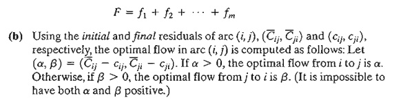
 The backtracking process of step 4 is invoked when the algorithm becomes "deadended" at an intermediate node. The flow adjustment in step 5 can be explained via the simple flow  network in Figure 6.30. Network (a)  gives  the first  breakthrough path N l  =  {I, 2, 3, 4} with its maximum flow It =  5. Thus, the residuals of each of arcs (1, 2), (2,3), and (3,4) are changed from (5,0) to (0,5), per step 5. Network (b) now gives the second breakthrough path N2  = {I, 3, 2, 4} with f2  = 5. After making the necessary flow adjustments, we get network (c), where no further breakthroughs are possible. What happened in the transition from (b) to (c) is nothing but a cancellation of a previously committed flow in the direction 2 -> 3. The algorithm is able to "remember" that

a flow from 2 to 3 has been committed previously only because we have increased the capacity in the reverse direction from 0 to 5 (per step 5).

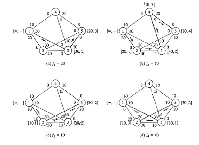
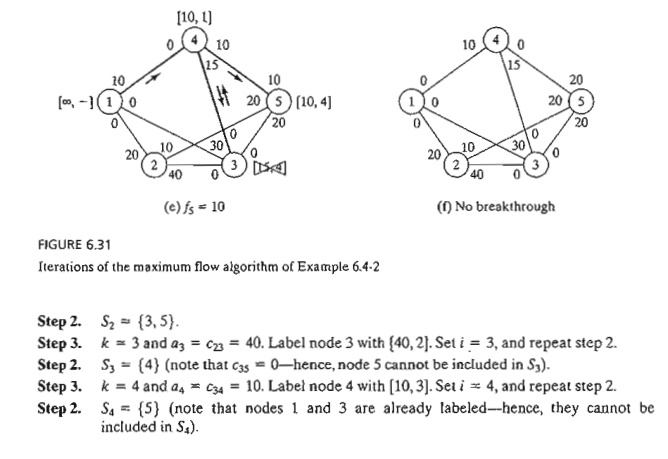
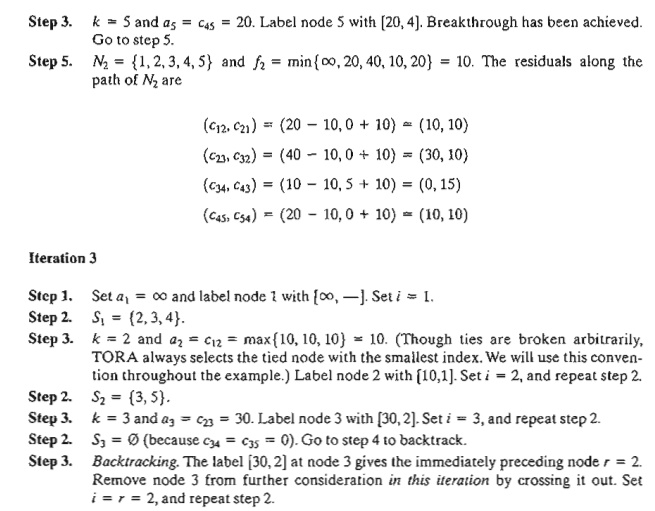
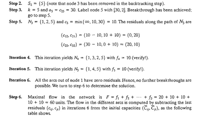
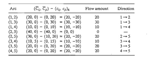
Example 6.4-2

Determine the maximal flow in the network of Example 6.4-1 (Figure 6.29). Figure 6.31 provides a graphical summary of the iterations of the algorithm. You will find it helpful to compare the description of the iterations with the graphical summary.

PROBLEM SET 6.4B

*1.  In Example 6.4-2,

a)     Determine the surplus capacities for all the arcs.

b)    Determine the amount of flow through nodes 2,3, and 4.

c)     Can the network flow be increased by increasing the capacities in the directions 3 ->  5 and 4-> 5?

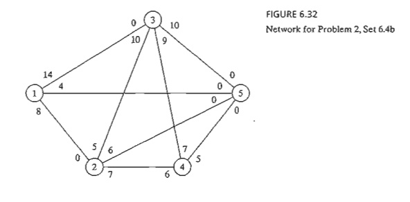
2. Determine the maximal flow and the optimum flow in each arc for the network in Figure 6.32.

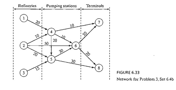
3. Three refineries send a gasoline product to two distribution terminals through a pipeline network. Any demand that cannot be satisfied through the network is acquired from other sources. The pipeline network is served by three pumping stations, as shown in Figure 6.33. The product flows in the network in the direction shown by the arrows. The capacity of each pipe segment (shown directly on the arcs) is in million bbl per day. Determine the following:

                                                                   i.      The daily production at each refinery that matches the maximum capacity of the net-work.

                                                                 ii.      The daily demand at each terminal that matches the maximum capacity of the net-work.

                                                              iii.      The daily capacity of each pump that matches the maximum capacity of the network.

4. Suppose that the maximum daily capacity of pump 6 in the network of Figure 6.33 is lim-ited to 50 million bbl per day. Remodel the network to include this restriction. Then determine the maximum capacity of the network.

5. Chicken feed is transported by trucks from three silos to four farms. Some of the silos can-not ship directly to some of the farms. The capacities of the other routes are limited by the number of trucks available and the number of trips made daily. The following table shows the daily amounts of supply at the silos and demand at the farms (in thousands of pounds). The cell entries of the table specify the daily capacities of the associated routes.

(a) Determine the schedule that satisfies the most demand.

(b) Will the proposed schedule satisfy all the demand at the farms?

6. In Problem 5, suppose that transshipping is allowed between silos 1 and 2 and silos 2 and 3. Suppose also that transshipping is allowed between farms 1 and 2,2 and 3, and 3 and 4. The maximum two-way daily capacity on the proposed transshipping routes is 50 (thousand) lb. What is the effect of transshipping on the unsatisfied demands at the farms?

*7. A parent has five (teenage) children and five household chores to assign to them. Past experience has shown that forcing chores on a child is counterproductive. With this in mind, the children are asked to list their preferences among the five chores, as the following table shows:

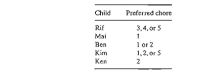
The parent's modest goal now is to finish as many chores as possible while abiding by the children's preferences. Determine the maximum number of chores that can be completed and the assignment of chores to children.

8. Four factories are engaged in the production of four types of toys. The following table lists the toys that can be produced by each factory.

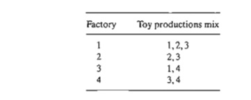
All toys require approximately the same per-unit labor and material. The daily capaci-ties of the four factories are 250,180,300, and 100 toys, respectively. The daily demands for the four toys are 200, 150, 350, and 100 units, respectively. Determine the factories' production schedules that will most satisfy the demands for the four toys.

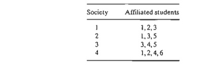
9. The academic council at the U of A is seeking representation from among six students who are affiliated with four honor societies. The academic council representation includes three areas: mathematics, art, and engineering. At most two students in each area can be on the council. The following table shows the membership of the six students in the four honor societies:

The students who are skilled in the areas of mathematics, art, and engineering are shown in the following table:

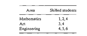
A student who is skilled in more than one area must be assigned exclusively to one area only. Can all four honor societies be represented on the council?

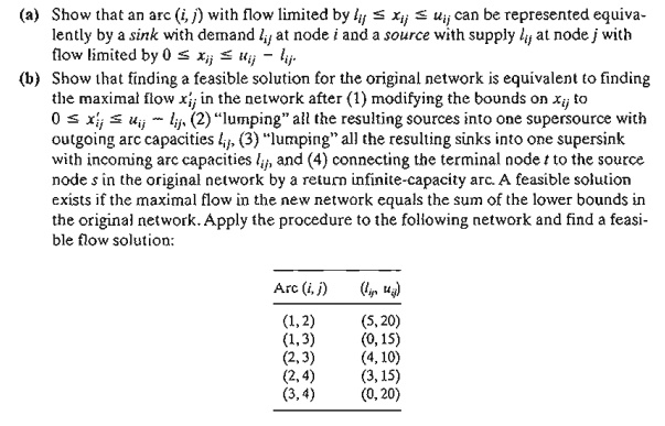
10. Maximal/minimal flow in networks with lower bounds. The maximal flow algorithm given in this section assumes that all the arcs have zero lower bounds. In some models, the lower bounds may be strictly positive, and we may be interested in finding the maximal or minimal flow in the network (see case 6-3 in Appendix E). The presence of the lower bound poses difficulty because the network may not have a feasible flow at all. The objective of this exercise is to show that any maximal and minimal flow model with positive lower bounds can be solved using two steps.

Step 1.Find an initial feasible solution for the network with positive lower bounds.

Step 2. Using the feasible solution in step 1, find the maximal or minimal flow in the original network.

(c) Use the feasible solution for the network in (b) together with the maximal flow algorithm to determine the minimal flow in the original network. (Hint: First compute the residue network given the initial feasible solution. Next, determine the maximum flow from the end node to the start node. This is equivalent to finding the maximum flow that should be canceled from the start node to the end node. Now, combining the fea-sible and maximal flow solutions yields the minimal flow in the original network.)

(d) Use the feasible solution for the network in (b) together with the maximal flow model to determine the maximal flow in the original network. (Him: As in part (c), start with the residue network. Next apply the breakthrough algorithm to the result-ing residue network exactly as in the regular maximal flow model.)

3. Linear Programming Formulation of Maximal Flow Mode

Define x_ij as the amount of flow in arc (i,j) with capacity c_ij . The objective is to determine x_ij for all i and j that will maximize the flow between start node s and terminal node t subject to flow restrictions (input flow = output flow) at all but nodes s and t.

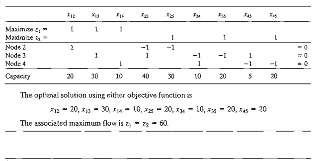
Example 6.4-3

In the maximal flow model of Figure 6.29 (Example 6.4-2), s = 1 and t = 5. The following table summarizes the associated LP with two different, but equivalent, objective functions depending on whether we maximize the output from start node 1 (= z.) or the input to terminal node

Solver Moment

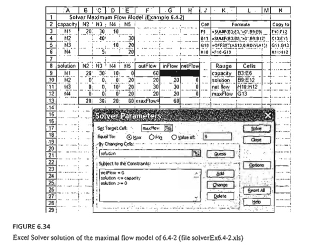
Figure 6.34 gives the Excel Solver model for the maximum flow model of Example 6.4-2 (file solverEx6.4-2.xls). The general idea of the model is similar to that used with the shortest-route model, which was detailed following Example 6.3-6. The main differences are: (1) there are no flow equations for the start node 1 and end node 5, and (2) the ob-jective is to maximize the total outflow at start node 1 (F9) or, equivalently, the total in-flow at terminal node 5 (G13). File solverEx6.4-2.xls uses G13 as the target cell. You are encouraged to execute the model with F9 as the target cell.

AMPLMoment

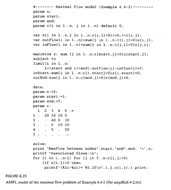
Figure 6.35 provides the AMPL model for the maximal flow problem. The data applies to Example 6.4-2 (file ampIEx6.4-2.txt). The overall idea of determining the input and output flows at a node is similar to the one detailed following Example 6.3-6 of the shortest-route model (you will find it helpful to review files amplEx6.3-6a.txt and ampIEx6.3-6b.txt first). However, because the model is designed to find the maximum flow between any two nodes, start and end, two additional constraints are needed to ensure that no flow enters start and no flow Leaves end. Constraints inStart and

QutEnd in the model ensure this result. These two constraints are not needed when start=l and end=5 because the nature of the data guarantees the desired result. However, for start=3, node 3 allows both input and output flow (arcs 4-3 and 3-4) and, hence, constraint inS tart is needed (try the model without inStart!).

The objective function maximizes the sum of the output flow at node start. Equivalently, we can choose to maximize the sum of the input flow at node end. The model can find the maximum flow between any two designated start and end nodes in the network.

PROBLEM SET 6.4C

1. Model each of the following problems as a linear program, then solve using Solver and AMPL.

a.     Problem 2, Set 6.4b.

b.     Problem 5,Set 6.4b

c.      Problem 9, Set 6.4b.

2. Jim lives in Denver, Colorado, and likes to spend his annual vacation in Yellowstone National Park in Wyoming. Being a nature lover, Jim tries to drive a different scenic route each year. After consulting the appropriate maps, Jim has represented his preferred routes between Denver (D) and Yellowstone (Y) by the network in Figure 6.36. Nodes 1 through 14 represent intermediate cities. Although driving distance is not an issue,Jim's stipulation is that selected routes between D and Y do not include any common cities.

Determine (using AMPL and Solver) all the distinct routes available to Jim. (Hint: Modify the maximal flow LP model to determine the maximum number of unique paths between D and Y.)

3. (Gueret and Associates, 2002, Section 12.1) A military telecommunication system con-necting 9 sites is given in Figure 6.37. Sites 4 and 7 must continue to communicate even if as many as three other sites are destroyed by enemy actions. Does the present communication network meet this requirement? Use AMPL and Solver to work out the problem.