Components at an Arbitrary Orientation (Tensor Transformation)

Components at an Arbitrary Orientation (Tensor Transformation)

In the previous sections, for convenience, the strain and stress tensors have been developed in Cartesian, x, y, z, coordinates drawn with the x and y horizontal and vertical in the 'plane-of-the-paper.' We know, however, that this orientation at a point is completely arbitrary, as is implied by indicial notation where ij can take on values r, ?, ? or a,b,c, or 1,2,3, or x,y,z depending on the global coordinate system we choose. Second-order tensors (diadics) are simply a combination of nine vector component magnitudes (3 vectors) on orthogonal planes. Thus, as we would expect for vectors, each component transforms into a new value as the coordinate rotates by sine and/or cosine relationships. We will derive them for the stress tensor because most of us find it easiest to visualize forces and use equilibrium arguments. The results are completely general, however, and apply to any symmetric tensor. In par ticular, they apply to the strain tensor where the normal components

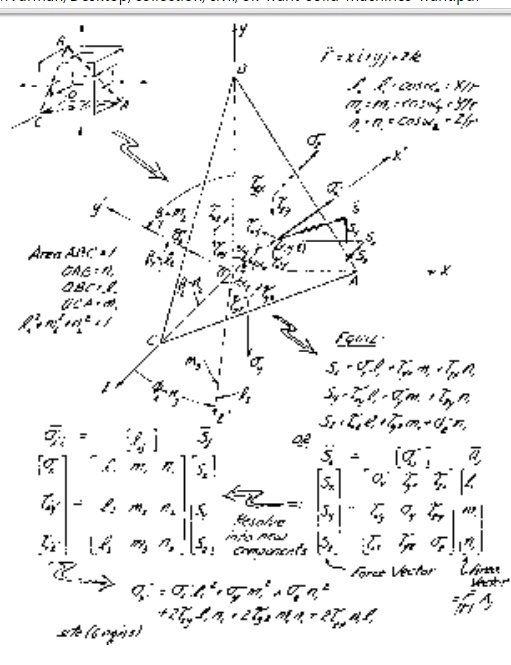
Consider a new orientation x',y', z' which would result if the 'stress block' were sliced out of the structural blob in a different orientation ( n correspond-ing to x' in Figure 2.3e). In other words the new x' coordinate axis is rotated ?_x, ?_y, ?_z, as shown in Figure 2.4. Rather than use the angles directly, let their

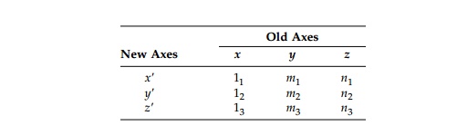
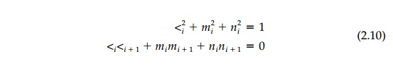
The direction cosines are not mutually independent but can be reduced to three independent variables by six relationships:

The direction cosines also represent the areas of the faces of the tetrahe-dron. Therefore, referring to Figure 2.4, the total force S Bar on the new exposed x' face ABC with area 1.0 can be found by equilibrium to be:

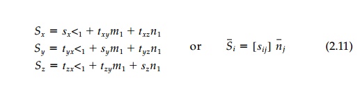
where n_j  has the direction cosines l₁, m₁, n₁ as components.

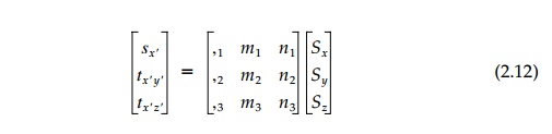
As the final step, the force S on the x' plane can be 'dissolved' back into the new stress components ?_{x_}, ?_{x_y_}, ?_{x_z_} by again using the direction cosines:

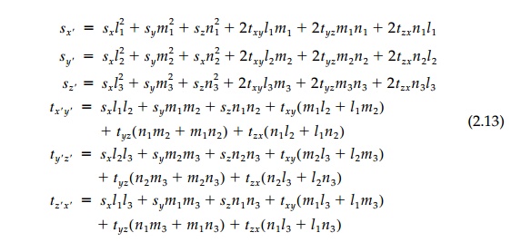
This same procedure of cutting new tetrahedrons to expose faces with normals in the y' and z' directions will produce the complete set of 3D

transformations in Equation (2.13) as follows:

In indicial notation these transformation equations, which provide an ana-lytic test for second-order tensors, can be written:

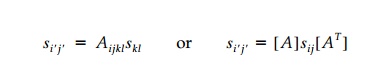
showing that it takes a fourth-order tensor (made up of direction cosines) to transform a second-order tensor. In practice it is more revealing and often easier to accomplish the transformation in two stages rather than use Equa-tion (2.13) directly. First the 'principal' state is found and the axes are then rotated, if necessary, from there. Usually the engineer is most interested in the principal state anyway since, in this orientation, the shear stresses are zero and normal components take on their maximum and minimum values.

Invariants and Principal Orientation

A vector can be plotted on paper in its fundamental or principal form as an arrow with magnitude and direction. It can then be decomposed into endless sets of different x', y', z' components analytically or graphically by the paral-lelogram law (cosines), each orthogonal set representing the same vector. Equations (2.13) demonstrate the same essential property for tensors (which are, after all, just a combination of vectors) but there is no neat graphical rep-resentation in 3D, or at least it is not directly apparent. At the same time we know that 'the point' cannot feel anything different between one set of com-ponents or another equivalent set at some new orientation. Thus, although a tensor can be decomposed into endless sets of different vector components at a point, the body must actually feel the same effect regardless of our orienta-tion when looking at it.

This fundamental description of a tensor, not tied to any particular coordi-nate system, must involve the 'invariant' coefficients of the characteristic equation for determining the principal values (or eigenvalues) and their directions as presented in Chapter 1 (for the general linear finite displace-ment tensor). For the stress tensor, this characteristic Equation (1.10), is:

The three roots (values of ?) are the principal stresses called ?₁, ?₂, ?₃ and they are real since the stress tensor (or the strain tensor) is symmetric. It is in this principal orientation of orthogonal axes 1, 2, 3, that the tensor is diago-nalized (no ? or ? ) and thus, in a principal direction (say of ?₁), Equation (2.11) takes the form:

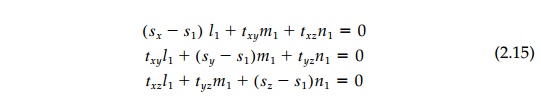
which, with the identity l²₁ + n²₁ + m²₁ = 1, can be solved for the direction cosines (the eigenvector) giving the orientation of the 1 or major principal axis. The same procedure is followed with ?₂ to find l₂, m₂, n₂ and ?₃ to find l₃, m₃, n₃ giving the directions of the intermediate and minor principal stresses respectively.

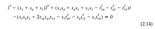
But Equation (2.14) is true for any choice of axes and therefore the coeffi-cients must be the same in any coordinate system. These coefficients then are the invariants:

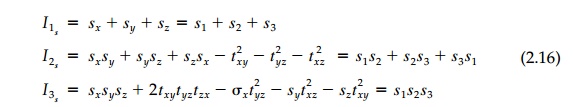
They are scalers and must be the 'fundamental essence' of a stress tensor. The corresponding invariants of the strain tensor can be deduced by anal-

ogy to be:

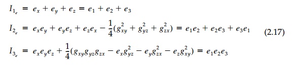
or we could write them for moment of inertia, electromagnetic flux, or any second-order tensor.