Linear Programming Formulation of the Shortest-Route Problem

Linear Programming Formulation of the Shortest-Route Problem

This section provides an LP model for the shortest-route problem. The model is gen-eral in the sense that it can be used to find the shortest route between any two nodes in the network. In this regard, it is equivalent to Floyd's algorithm.

Suppose that the shortest-route network includes n nodes and that we desire to determine the shortest route between any two nodes sand t in the network. The LP assumes that one unit of flow enters the network at node s and leaves at node t.

Define

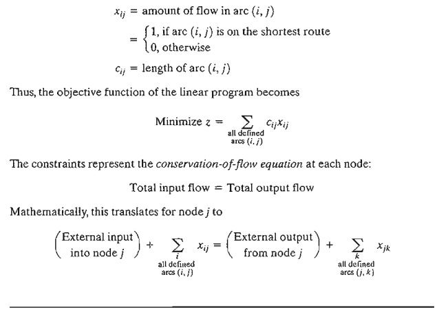
Example 6.3-6

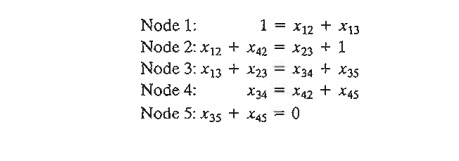
Consider the shortest-route network of Example 6.3-4. Suppose that we want to determine the shortest route from node 1 to node 2-that is, s = 1 and t = 2. Figure 6.24 shows how the unit of flow enters at node 1 and leaves at node 2.

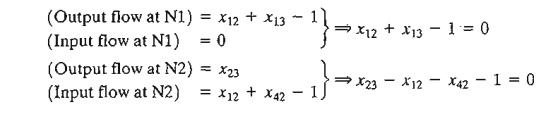
We can see from the network that the flow-conservation equation yields

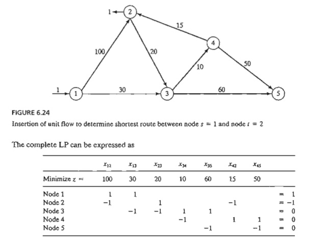
Notice that column x_ij has exactly one "1" entry in row i and one "-I" entry in row j, a typical property of a network LP.

The optimal solution (obtained by TORA, file toraEx6.3-6.txt) is

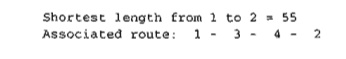
This solution gives the shortest route from node 1 to node 2 as 1 -> 3-> 4 -> 2, and the associated distance is z = 55 (miles).

PROBLEM 6.30

1. In Example 6.3-6, use LP to determine the shortest routes between the following pairs of nodes:

*(a) Node 1 to node 5.

(b) Node 2 to node 5.

Solver Moment

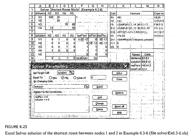
Figure 6.25 provides the Excel Solver spreadsheet for finding the shortest route between start node Nl and end node N2 of Example 6.3-6 (file solverEx6.3-6.xls). The input data of the model is the distance matrix in cells B3:E6. Node Nl has no column because it has no incoming arcs, and node N5 has no row because it has no outgoing arcs. A blank entry means that the corresponding arc does not exist. Nodes Nl and N2 are designated as the start and end nodes by entering 1 in F3 and B7, respectively. These designations can be changed simply by moving the entry 1 to new cells. For example, to fmd the shortest route from node N2 to node N4, we enter 1 in each of F4 and D7.

The solution of the model is given cells B9:E12. A cell defines a leg connecting its designated nodes. For example, cell C10 defines the leg (N2, N3), and its associated variable is x₂₃. A cell variable x_ij = 1 if its leg (Ni, Nj) is on the route. Otherwise, its value is zero.

With the distance matrix given by the range B3:E6 (named distance) and the solution matrix given by the range B9:E12 (named solution), the objective function is computed in cell G14 as =SUMPRODUCT(B3: E6,B9: E12) or, equivalently, =SUMPRODUT (distance, solution). You may wonder about the significance of the blank entries (which default to zero by Excel) in the distance matrix and their impact on the definition of the objective function. This point will be addressed shortly, after we have shown how the corresponding variables are totally excluded from the constraints of the problem.

As explained in the LP of Example 6.3-6, the constraints of the problem are of the general form:

(Output flow) - (Input flow) = 0

This definition is adapted to the spreadsheet layout by incorporating the external unit flow, if any, directly in either Output flow or Input flow of the equation. For example, in Example 6.3-6, an external flow unit enters at Nl and leaves at N2. Thus, the associated constraints are given as

Looking at the spreadsheet in Figure 6.25, the two constraints are expressed in terms of the cells as

(Output flow at Nl)=B9+C9-F3

(Input flow at Nl) =0

(Output flow at N2)=CIO

(Input flow at N2) =89+812-B7

To identify the solution cells in the range B9:E12 that apply to each constraint, we note that a solution cell forms part of a constraint only if it has a positive entry in the distance matrix. Thus, we use the following formulas to identify the output and input flows for each node:

1.    Output flow: Enter=SUMIF (83; E3) ">0" ,   B9: E9) -F3  in cell F9 and copy it in cells F10:F12.

2. Input Flow: Enter=sUMIF (B3 ; B6 , ">0" , 89 : 812) -87 in cell B14 and copy it in cells CI4:EI4.

3. Enter =OFFSET (A$14, 0,I ROW (AI) ) in cell GI0 and copy it in cells Gl1:G13 to transpose the input flow to column G.

4. Enter 0 in each of G9 and F13 to indicate that Nl has no input flow and N5 has no output flow (per spreadsheet definitions).

5. Enter =F9-G9 in cell H9 and copy it in cells HIO:H13 to compute the net flow.

The spreadsheet is now ready for the application of Solver as shown in Figure 6.25. There is one curious occurrence though: When you define the constraints within the Solver Parameters dialogue box as outFlow = inFlow, Solver does not locate a feasi-ble solution, even after making adjustments in precision in the Solver Option box. (To reproduce this experience, solution cells B9:E12 must be reset to zero or blank.) More curious yet, if the constraints are replaced with inFlow = outFlow, the optimum solu-tion is found. In file solverEx6.3-6.xls, we use the nefFlow range in cells H9:Hl2 and express the constraint as netFlow = 0 with no problem. It is not clear why this pecu-liarity occurs, but the problem could be related to roundoff error.

The output in Figure 6.25 yields the solution (NI-N3 = 1, N3-N4 = 1, N4-N2 = 1) with a total distance of 55 miles. This means that the optimal route is 1 ->  3 ->  4 -> 2.

Remarks. In most textbooks, the network is defined by its explicit arcs (node i, node j, distance ), a lengthy and inconvenient process that may not be practical when the number of arcs is large. Our model is driven primarily by the compact distance matrix, which is all we need to develop the flow constraints. It may be argued that our model deals with (n - 1 X n - 1 )x_ij-variables, which could be much larger than the number of variables associated with the arcs of the model (for instance, Example 6.3-6 has 7 arcs and hence 7 x_ij- variables, as opposed to 4 X 4 = 16 in our formulation). Keep in mind that these additional variables appear only in the objective function and with zero coefficients (blank entries) and that the flow constraints are exactly the same as in other presentations (per the SUMIF function). As a result, pre-solvers in commercial software will spot this "oddity" and automatically exclude the additional variables prior to ap-plying the simplex method, with no appreciable computational overhead.

AMPLMoment

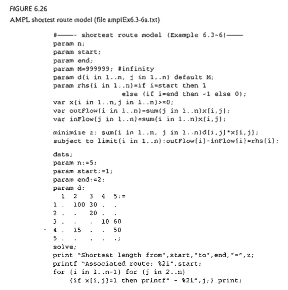
Figure 6.26 provides the AMPL model for solving Example 6.3-6 (file ampIEx6.3-6a.txt). The variable x [i, j] assumes the value 1 if arc [i, j] is on the shortest route and 0 otherwise. The model is general in the sense that it can be used to find the shortest route between any two nodes in a problem of any size.

As explained in Example 6.3-6, AMPL treats the problem as a network in which an external flow unit enters and exits at specified start and end nodes. The main input data of the model is an n X n matrix representing the distance d {i, j] of the arc joining nodes i and j. Per AMPL syntax, a dot entry in d (i , j] is a placeholder that signifies

that no distance is specified for the corresponding arc. In the model, the dot entry is overridden by the infinite distance M (= 999999) in param d {i in 1 ... n, j in 1 ... n} default M; which will convert it into an infinite-distance route. The same result could be achieved by replacing the dot entry (.) with 999999 in the data section, which, in addition to "cluttering" the data, is inconvenient.

The constraints represent flow conservation through each node:

(Input flow)  - (Output flow)  = (External flow)

From x [i, j], we can define the input and output flow for node i using the statements

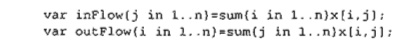
The left-hand side of the constraint i is thus given as outFlow [i] -inFlow [i].

The right-hand side of constraint i (external flow at node i) is defined as

(See Section A.3 for details of if then else.) With this statement, specifying start and end nodes automatically assigns 1, - 1, or 0 to rhs, the right-hand side of the constraints.

The objective function seeks the minimization of the sum of d [i, j ] * x [i, j ] over all i and j.

In the present example, start=1 and end=2, meaning that we want to determine the shortest route from node 1 to node 2. The associated output is

Remarks. The AMPL model as given in Figure 6.26 has one flaw: The number of active variables x_ij is n² , which could be significantly much larger than the actual number of (positive-distance) arcs in the network, thus resulting in a much larger problem. The reason is that the model accounts for the nonexisting arcs by assigning them an in-finite distance M (= 999999) to guarantee that they will be zero in the optimum solution. This situation can be remedied by using a subset of {i in 1 .. n, j in 1 .. n} that excludes nonexisiting arcs, as the following statement shows:

(See Section AA for the use of conditions to define subsets.) The same logic must be applied to the constraints as well by using the following statements:

File amplEx6.36b.txt gives the complete model.

PROBLEM 6.3E

1. Modify solverEx6.3-6.xls to find the shortest route between the following pairs of nodes:

a. Node 1 to node 5.

b. Node 4 to node 3.

2. Adapt amplEx6.3-6b.txt for Problem 2, Set 6.3a, to find the shortest route between node 1 and node 7. The input data must be the raw probabilities. Use AMPL programming facilities to print/display the optimum transmission route and its success probability.