Crossing Over

Crossing Over

Crossing over is a biological process that produces new combination of genes by inter-changing the corresponding segments between non-sister chromatids of homologous pair of chromosomes. The term 'crossing over' was coined by Morgan (1912). It takes place during pachytene stage of prophase I of meiosis. Usually crossing over occurs in germinal cells during gametogenesis. It is called meiotic or germinal crossing over. It has universal occurrence and has great significance. Rarely, crossing over occurs in somatic cells during mitosis. It is called somatic or mitotic crossing over.

1. Mechanism of Crossing Over

Crossing over is a precise process that includes stages like synapsis, tetrad formation, cross over and terminalization.

(i) Synapsis

Intimate pairing between two homologous chromosomes is initiated during zygotene stage of prophase I of meiosis I. Homologous chromosomes are aligned side by side resulting in a pair of homologous chromosomes called bivalents. This pairing phenomenon is called synapsis or syndesis. It is of three types,

1. Procentric synapsis: Pairing starts from middle of the chromosome.

2. Proterminal synapsis: Pairing starts from the telomeres.

3. Random synapsis: Pairing may start from anywhere.

(ii) Tetrad Formation

Each homologous chromosome of a bivalent begin to form two identical sister chromatids, which remain held together by a centromere. At this stage each bivalent has four chromatids. This stage is called tetrad stage.

(iii) Cross Over

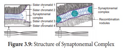
After tetrad formation, crossing over occurs in pachytene stage. The non-sister chromatids of homologous pair make a contact at one or more points. These points of contact between non-sister chromatids of homologous chromosomes are called Chiasmata (singular-Chiasma). At chiasma, cross-shaped or X-shaped structures are formed, where breaking and rejoining of two chromatids occur. This results in reciprocal exchange of equal and corresponding segments between them. A recent study reveals that synapsis and chiasma formation are facilitated by a highly organised structure of filaments called Synaptonemal Complex (SC) (Figure 3.9). This synaptonemal complex formation is absent in some species of male Drosophila hence crossing over does not takes place.

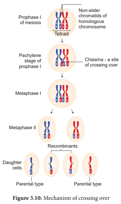
(iv) Terminalisation

After crossing over, chiasma starts to move towards the terminal end of chromatids. This is known as terminalisation. As a result, complete separation of homologous chromosomes occurs. (Figure 4.10)

2. Types of Crossing Over

Depending upon the number of chiasmata formed crossing over may be classified into three types. (Figure 3.11)

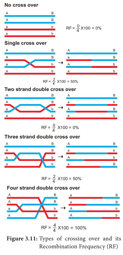
1. Single cross over: Formation of single chiasma and involves only two chromatids out of four.

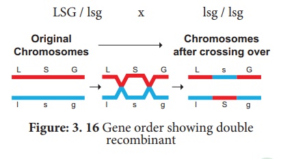
2. Double cross over: Formation of two chiasmata and involves two or three or all four strands

3. Multiple cross over: Formation of more than two chiasmata and crossing over frequency is extremely low.

3. Importance of Crossing Over

Crossing over occurs in all organisms like bacteria, yeast, fungi, higher plants and animals. Its importance is

·         Exchange of segments leads to new gene combinations which plays an important role in evolution.

·         Studies of crossing over reveal that genes are arranged linearly on the chromosomes.

·         Genetic maps are made based on the frequency of crossing over.

·         Crossing over helps to understand the nature and mechanism of gene action.

·         If a useful new combination is formed it can be used in plant breeding.

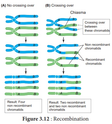
4.  Recombination

Crossing over results in the formation of new combination of characters in an organism called recombinants. In this, segments of DNA are broken and recombined to produce new combinations of alleles. This process is called Recombination. (Figure 3.12)

The widely accepted model of DNA recombination during crossing over is Holliday’s hybrid DNA model. It was first proposed by Robin Holliday in 1964. It involves several steps. (Figure 3.13)

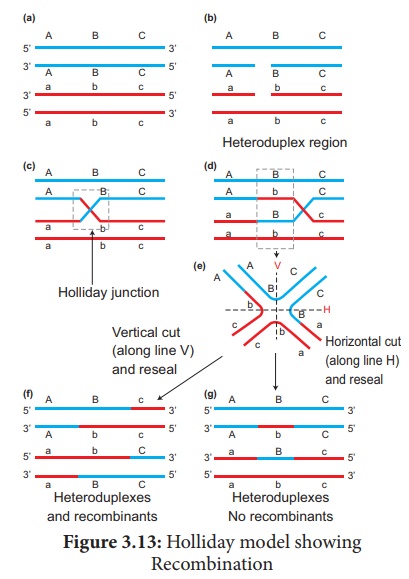
1.     Homologous DNA molecules are paired side by side with their duplicated copies of DNAs

2.     One strand of both DNAs cut in one place by the enzyme endonuclease.

3.     The cut strands cross and join the homologous strands forming the Holliday structure or Holliday junction.

4.     The Holliday junction migrates away from the original site, a process called branch migration, as a result heteroduplex region is formed.

5.     DNA strands may cut along through the vertical (V) line or horizontal (H) line.

6.     The vertical cut will result in hetero duplexes with recombinants.

7.     The horizontal cut will result in hetero duplex with non recombinants.

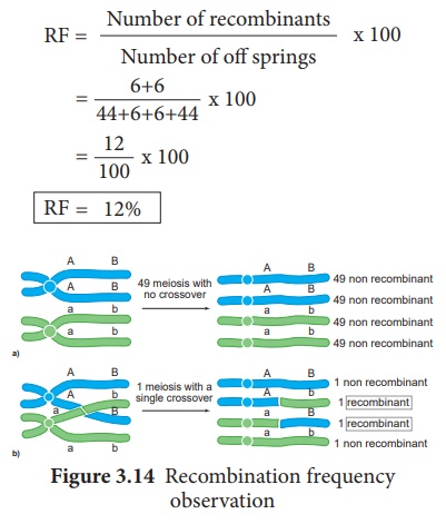
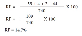
Calculation of Recombination Frequency (RF)

The percentage of recombinant progeny in a cross is called recombination frequency. The recombination frequency (cross over frequency) (RF) is calculated by using the following formula. The data is obtained from alleles in coupling configuration (Figure 3.14)

5. Genetic Mapping

Genes are present in a linear order along the chromosome. They are present in a specific location called locus (plural: loci). The diagrammatic representation of position of genes and related distances between the adjacent genes is called genetic mapping. It is directly proportional to the frequency of recombination between them. It is also called as linkage map. The concept of gene mapping was first developed by Morgan’s student Alfred H Sturtevant in 1913. It provides clues about where the genes lies on that chromosome.

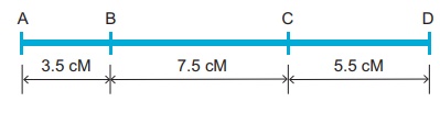
Map distance

The unit of distance in a genetic map is called a map unit (m.u). One map unit is equivalent to one percent of crossing over (Figure 4. ). One map unit is also called a centimorgan (cM) in honour of T.H. Morgan. 100 centimorgan is equal to one Morgan (M). For example: A distance between A and B genes is estimated to be 3.5 map units. It is equal to 3.5 centimorgans or 3.5 % or 0.035 recombination frequency between the genes.

Genetic maps can be constructed from a series of test crosses for pairs of genes called two point crosses. But this is not efficient because double cross over is missed.

Three point test cross

A more efficient mapping technique is to construct based on the results of three-point test cross. It refers to analyzing the inheritance patterns of three alleles by test crossing a triple recessive heterozygote with a triple recessive homozygote. It enables to determine the distance between the three alleles and the order in which they are located on the chromosome. Double cross overs can be detected which will provide more accurate map distances.

Three-point test cross can be best understood by considering following an example.

In maize (corn), the three recessive alleles are

1.  l for lazy or prostrate growth habit

2.  g for glossy leaf

3.  s for sugary endosperm

These three recessive alleles (l g s) are crossed with wild type dominant alleles (L G S).

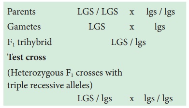
Parents       LGS / LGS  x        lgs / lgs

Gametes      LGS  x        lgs

F1 trihybrid          LGS / lgs

Test cross

(Heterozygous F1 crosses with

triple recessive alleles)

 LGS / lgs    x        lgs / lgs

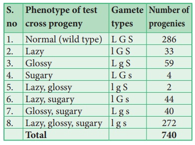
This trihybrid test cross produces 8 different types (23=8) of gametes in which 740 progenies are observed. The following table shows the result obtained from a test cross of corn with three linked genes.

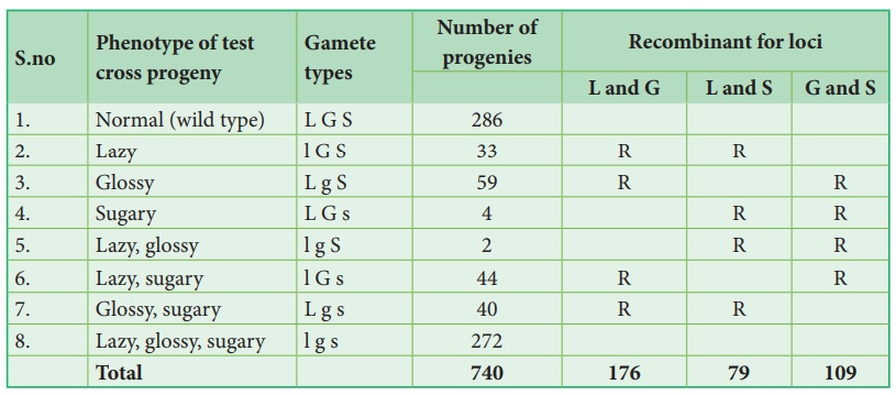
The analysis of a three-point cross:

From the above result, we must be careful to observe parental (P) and recombinant (R) types. First note that parental genotypes for the triple homozygotes are L G S and l g s, then analyse two recombinant loci at a time orderly L G/ l g, L S/ l s and G S/ g s. In this any combination other than these two constitutes a recombinant (R).

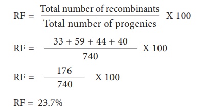
Let’s analyse the loci of two alleles at a time starting with L and G Since the L G and l g parental genotypes the recombinants will be L g and l G. The Recombinant frequency (RF) for these two alleles can be calculated as follows

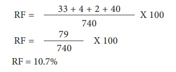
For L and S loci, the recombinants are L s and l S. The Recombinant frequency (RF) will be as follows

For G and S loci, the recombinants are G s and g S. The Recombinant frequency (RF) will be as follows

All the loci are linked, because all the RF values are considerably less than 50%. In this L G loci show highest RF value, they must be farthest apart. Therefore, the S locus must lie between them. The order of genes should be l s g. A genetic map can be drawn as follows: (Figure 3.15)

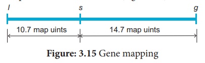
A final point note that two smaller map distances, 10.7 m.u and 14.7., is add up to 25.4 m.u., which is greater than 23.7 m.u., the distance calculated for l and g. we must identify the two least number of progenies (totaling 8) in relation to recombination of L and G. These two least progenies are double recombinants arising from double cross over. The two least progenies not only counted once should have counted each of them twice because each represents a double recombinant progeny.

Hence, we can correct the value adding the numbers 33+59+44+40+4+4+2+2=188. Of the total of 740, this number exactly 25.4 %, which is identical with the sum of two component values.

The test cross parental combination can be re written as follows:

Uses of genetic mapping

·         It is used to determine gene order, identify the locus of a gene and calculate the distances between genes.

·         They are useful in predicting results of dihybrid and trihybrid crosses.

·         It allows the geneticists to understand the overall genetic complexity of particular organism.