Synchronization Between Parallel Loops

Synchronization Between Parallel Loops

1 A Constant Number of Synchronizations

2 Program-Dependence Graphs

3 Hierarchical Time

4 The Parallelization Algorithm

5 Exercises for Section 11.8

Most programs have no parallelism if we do not allow processors to perform any synchronizations. But adding even a small constant number of synchronization operations to a program can expose more parallelism. We shall first discuss parallelism made possible by a constant number of synchronizations in this section and the general case, where we embed synchronization operations in loops, in the next.

1. A Constant Number of Synchronizations

Programs with no synchronization-free parallelism may contain a sequence of loops, some of which are parallelizable if they are considered independently. We can parallelize such loops by introducing synchronization barriers before and after their execution. Example 11.49 illustrates the point.

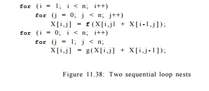
Example 1 1 . 4 9 : In Fig. 11.38 is a program representative of an ADI (Alter-nating Direction Implicit) integration algorithm. There is no synchronization-free parallelism. Dependences in the first loop nest require that each processor works on a column of array X; however, dependences in the second loop nest require that each processor works on a row of array X. For there to be no com-munication, the entire array has to reside on the same processor, hence there is no parallelism. We observe, however, that both loops are independently parallelizable.

One way to parallelize the code is to have different processors work on different columns of the array in the first loop, synchronize and wait for all processors to finish, and then operate on the individual rows. In this way, all the computation in the algorithm can be parallelized with the introduction of just one synchronization operation. However, we note that while only one synchronization is performed, this parallelization requires almost all the data in matrix X to be transferred between processors. It is possible to reduce the amount of communication by introducing more synchronizations, which we shall discuss in Section 11.9.9.

It may appear that this approach is applicable only to programs consisting of a sequence of loop nests. However, we can create additional opportunities for the optimization through code transforms. We can apply loop fission to decompose loops in the original program into several smaller loops, which can then be parallelized individually by separating them with barriers. We illustrate this technique with Example 11.50.

Example 1 1 . 5 0 :  Consider the following loop:

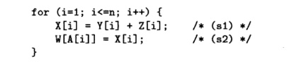
Without knowledge of the values in array A, we must assume that the access in statement s₂ may write to any of the elements of W. Thus, the instances of S2 must be executed sequentially in the order they are executed in the original program.

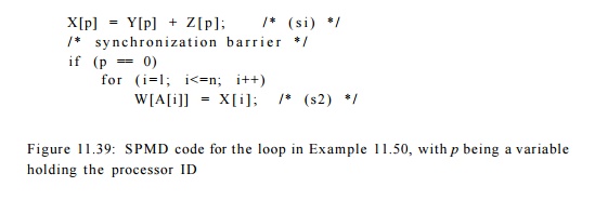
There is no synchronization-free parallelism, and Algorithm 11.43 will sim-ply assign all the computation to the same processor. However, at the least, instances of statement si can be executed in parallel. We can parallelize part of this code by having different processors perform difference instances of state-ment si. Then, in a separate sequential loop, one processor, say numbered 0, executes s₂, as in the SPMD code shown in Fig. 11.39. •

2. Program-Dependence Graphs

To find all the parallelism made possible by a constant number of synchroniza-tions, we can apply fission to the original program greedily. Break up loops into as many separate loops as possible, and then parallelize each loop indepen-dently.

To expose all the opportunities for loop fission, we use the abstraction of a program-dependence graph (PDG). A program dependence graph of a program

is a graph whose nodes are the assignment statements of the program and whose edges capture the data dependences, and the directions of the data dependence, between statements. An edge from statement si to statement s₂ exists whenever some dynamic instance of s1 shares a data dependence with a later dynamic instance of s2. 

 To construct the PDG for a program, we first find the data dependences between every pair of (not necessarily distinct) static accesses in every pair of (not necessarily distinct) statements. Suppose we determine that there is a dependence between access T1 in statement s1 and access T2 in statement s2. Recall that an instance of a statement is specified by an index vector i = [hih, • • • ,im] where ik is the loop index of the kth outermost loop in which the statement is embedded.

 1. If there exists a data-dependent pair of instances, ii of si and i2 of s2, and ii is executed before i2 in the original program, written ii ^ S l S 2 l2, then there is an edge from s1 to s2.

 2. Similarly, if there exists a data-dependent pair of instances, ii of si and i 2 of s2, and i 2 - < s i s 2 ii> then there is an edge from s2 to s1.

Note that it is possible for a data dependence between two statements si and s2 to generate both an edge from si to s2 and an edge from s2 back to s1.

 In the special case where statements si and s2 are not distinct, ii - < S l s 2 i 2 if and only if ii -< i2 (ii is lexicographically less than i 2 ) . In the general case, si and s2 may be different statements, possibly belonging to different loop nests.

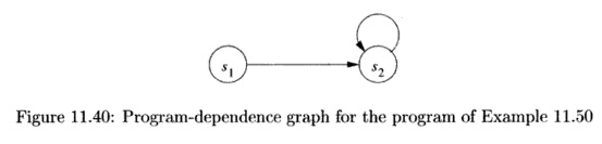
Example 1 1 . 5 1 : For the program of Example 11.50, there are no dependences among the instances of statement s1. However, the z'th instance of statement s2 must follow the ith instance of statement 81. Worse, since the reference Wp4[i]] may write any element of array W, the ith instance of s2 depends on all previous instances of s2. That is, statement s2 depends on itself. The PDG for the program of Example 11.50 is shown in Fig. 11.40. Note that there is one cycle in the graph, containing s2 only.

The program-dependence graph makes it easy to determine if we can split statements in a loop. Statements connected in a cycle in a PDG cannot be

split. If si —y s₂ is a dependence between two statements in a cycle, then some instance of si must execute before some instance of s₂, and vice versa. Note that this mutual dependence occurs only if si and s₂ are embedded in some common loop. Because of the mutual dependence, we cannot execute all instances of one statement before the other, and therefore loop fission is not allowed. On the other hand, if the dependence s± s₂ is unidirectional, we can split up the loop and execute all the instances of si first, then those of s₂.

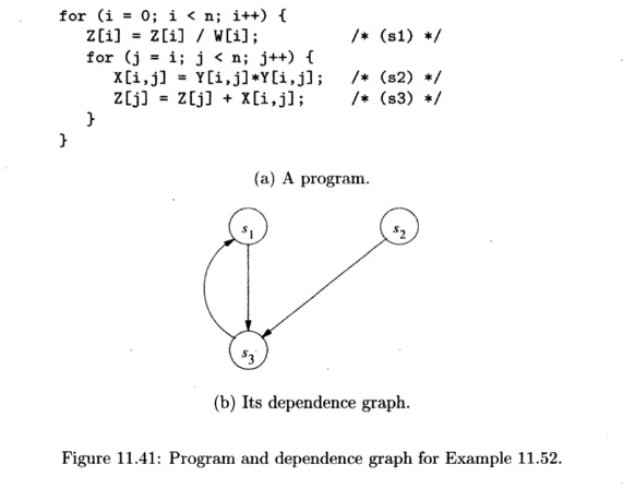
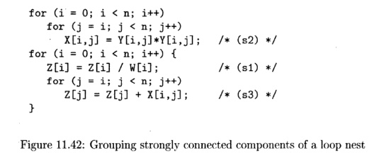
Example 1 1 . 5 2 : Figure  11.41(b)  shows the  program-dependence graph for the program o f Fig. 11.41(a).  Statements s ± and 5 3 belong t o a cycle in the graph and therefore cannot be placed in separate loops. We can, however, split statement s₂ out and execute all its instances before executing the rest of the computation, as in Fig. 11.42. The first loop is parallelizable, but the second is not. We can parallelize the first loop by placing barriers before and after its parallel execution.

3. Hierarchical Time

While the relation - < _{S l S 2} can be very hard to compute in general, there is a family of programs to which the optimizations of this section are commonly applied, and for which there is a straightforward way to compute dependencies. Assume that the program is block structured, consisting of loops and simple arithmetic operations and no other control constructs. A statement in the program is either an assignment statement, a sequence of statements, or a loop construct whose body is a statement. The control structure thus represents a hierarchy. At the top of the hierarchy is the node representing the statement of the whole program. An assignment statement is a leaf node. If a statement is a sequence, then its children are the statements within the sequence, laid out from left to right according to their lexical order. If a statement is a loop, then its children are the components of the loop body, which is typically a sequence of one or more statements.

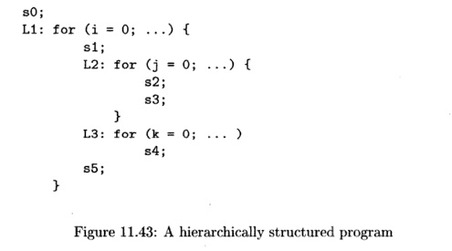
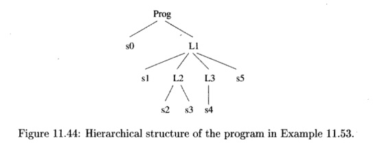
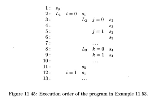
Example 1 1 . 5 3 : The hierarchical structure of the program in Fig. 11.43 is shown in Fig. 11.44. The hierarchical nature of the execution sequence is high lighted in Fig. 11.45. The single instance of s₀ precedes all other operations, because it is the first statement executed. Next, we execute all instructions from the first iteration of the outer loop before those in the second iteration and so forth. For all dynamic instances whose loop index i has value 0, the statements si, L₂, L₃, and s₅ are executed in lexical order. We can repeat the same argument to generate the rest of the execution order.

We can resolve the ordering of two instances from two different statements in a hierarchical manner. If the statements share common loops, we compare the values of their common loop indexes, starting with the outermost loop. As soon as we find a difference between their index values, the difference determines the ordering. Only if the index values for the outer loops are the same do we need to compare the indexes of the next inner loop. This process is analogous to how we would compare time expressed in terms of hours, minutes and seconds. To compare two times, we first compare the hours, and only if they refer to the same hour would we compare the minutes and so forth. If the index values are the same for all common loops, then we resolve the order based on their relative lexical placement. Thus, the execution order for the simple nested-loop programs we have been discussing is often referred to as  "hierarchical time." Let si  be a statement nested in a di-deep loop, and s2    in a d2 -deep loop,

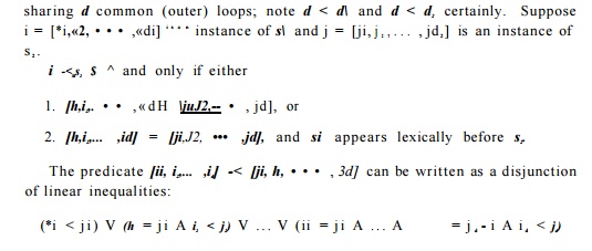
A PDG edge from si to s₂ exists as long as the data-dependence condition and one of the disjunctive clauses can be made true simultaneously. Thus, we may need to solve up to d or d + 1 linear integer programs, depending on whether si appears lexically before s₂, to determine the existence of one edge.

4. The Parallelization Algorithm

We now present a simple algorithm that first splits up the computation into as many different loops as possible, then parallelizes them independently.

Algorithm 11 . 5 4 : Maximize the degree of parallelism allowed by 0(1) syn-chronizations.

INPUT: A program with array accesses.

OUTPUT: SPMD code with a constant number of synchronization barriers.

METHOD:

1.          Construct the program-dependence graph and partition the statements into strongly connected components (SCC's). Recall from Section 10.5.8 that a strongly connected component is a maximal subgraph of the orig-inal whose every node in the subgraph can reach every other node.

2.          Transform the code to execute SCC's in a topological order by applying fission if necessary.

3.          Apply Algorithm 11.43 to each SCC to find all of its synchronization-free parallelism. Barriers are inserted before and after each parallelized SCC.

While Algorithm 11.54 finds all degrees of parallelism with 0(1) synchro-nizations, it has a number of weaknesses. First, it may introduce unnecessary synchronizations. As a matter of fact, if we apply this algorithm to a program that can be parallelized without synchronization, the algorithm will parallelize each statement independently and introduce a synchronization barrier between the parallel loops executing each statement. Second, while there may only be a constant number of synchronizations, the parallelization scheme may transfer a lot of data among processors with each synchronization. In some cases, the cost of communication makes the parallelism too expensive, and we may even be better off executing the program sequentially on a uniprocessor. In the fol-lowing sections, we shall next take up ways to increase data locality, and thus reduce the amount of communication.

5. Exercises for Section 11.8

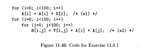
Exercise 11.8.1: Apply Algorithm 11.54 to the code of Fig. 11.46.

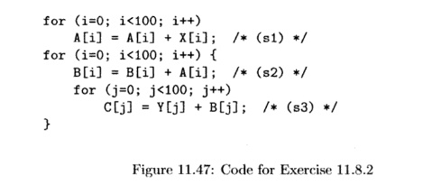
Exercise 1 1 . 8 . 2 : Apply Algorithm 11.54 to the code of Fig. 11.47.

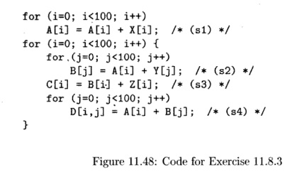
Exercise 11.8.3: Apply Algorithm 11.54 to the code of Fig. 11.48.