Iteration Spaces

Iteration Spaces

1 Constructing Iteration Spaces from Loop Nests

2 Execution Order for Loop Nests

3 Matrix Formulation of Inequalities

4 Incorporating Symbolic Constants

5 Controlling the Order of Execution

6 Changing Axes 798

7 Exercises for Section 11.3

The motivation for this study is to exploit the techniques that, in simple settings like matrix multiplication as in Section 11.2, were quite straightforward. In the more general setting, the same techniques apply, but they are far less intuitive. But by applying some linear algebra, we can make everything work in the general setting.

As discussed in Section 11.1.5, there are three kinds of spaces in our trans-formation model: iteration space, data space, and processor space. Here we start with the iteration space. The iteration space of a loop nest is defined to be all the combinations of loop-index values in the nest.

Often, the iteration space is rectangular, as in the matrix-multiplication example of Fig. 11.5. There, each of the nested loops had a lower bound of 0 and an upper bound of n — 1. However, in more complicated, but still quite realistic, loop nests, the upper and/or lower bounds on one loop index can depend on the values of the indexes of the outer loops. We shall see an example shortly.

1. Constructing Iteration Spaces from Loop Nests

To begin, let us describe the sort of loop nests that can be handled by the techniques to be developed. Each loop has a single loop index, which we assume is incremented by 1 at each iteration. That assumption is without loss of generality, since if the incrementation is by integer c > 1, we can always replace uses of the index i by uses of ci + a for some positive or negative constant a, and then increment i by 1 in the loop. The bounds of the loop should be written as affine expressions of outer loop indices.

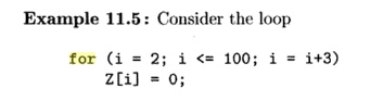
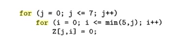
which increments i by 3 each time around the loop.  The effect is to set to 0 each of the elements Z[2], Z[5], Z [ 8 ] , . . . , Z[98]. We can get the same effect with:

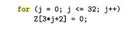
That is, we substitute 3j + 2 for i.  The lower limit i = 2 becomes j = 0 (just  solve 3j + 2 = 2 for j ) , and the upper limit i < 100 becomes j < 32 (simplify 3j + 2 < 100 to get j < 32.67 and round down because j has to be an integer).

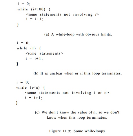
Typically, we shall use for-loops in loop nests.  A while-loop or repeat-loop can be replaced by a for-loop if there is an index and upper and lower bounds for the index, as would be the case in something like the loop of Fig. 11.9(a).

A for-loop like f o r  ( i = 0 ;  i<100;  i++) serves exactly the same purpose.

However, some while- or repeat-loops have no obvious limit. For example, Fig. 11.9(b) may or may not terminate, but there is no way to tell what condition on i in the unseen body of the loop causes the loop to break. Figure 11.9(c) is another problem case. Variable n might be a parameter of a function, for example. We know the loop iterates n times, but we don't know what n is at compile time, and in fact we may expect that different executions of the loop will execute different numbers of times. In cases like (b) and (c), we must treat the upper limit on i as infinity.

A <i-deep loop nest can be modeled by a dl-dimensional space. The dimen-sions are ordered, with the kth. dimension representing the kth nested loop, counting from the outermost loop, inward. A point (xi,x₂,... ,Xd) in this space represents values for all the loop indexes; the outermost loop index has value xi, the second loop index has value x₂, and so on. The innermost loop index has value x&.

But not all points in this space represent combinations of indexes that ac-tually occur during execution of the loop nest. As an affine function of outer loop indices, each lower and upper loop bound defines an inequality dividing the iteration space into two half spaces: those that are iterations in the loop (the positive half space), and those that are not (the negative half space). The conjunction (logical AND) of all the linear equalities represents the intersection of the positive half spaces, which defines a convex polyhedron, which we call the iteration space for the loop nest. A convex polyhedron has the property that if

two points are in the polyhedron, all points on the line between them are also in the polyhedron. All the iterations in the loop are represented by the points with integer coordinates found within the polyhedron described by the loop-bound inequalities. And conversely, all integer points within the polyhedron represent iterations of the loop nest at some time.

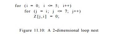
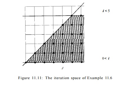
Example 1 1 . 6 :  Consider the 2-dimensional loop nest in Fig. 11.10.  We can model this two-deep loop nest by the 2-dimensional polyhedron shown in Fig. 11.11. The two axes represent the values of the loop indexes i and j. Index i can take on any integral value between 0 and 5; index j can take on any integral value such that i < j < 7.

Iteration Spaces and Array-Accesses

In the code of Fig. 11.10, the iteration space is also the portion of the array

A that the code accesses. That sort of access, where the array indexes are also loop indexes in some order, is very common. However, we should not confuse the space of iterations, whose dimensions are loop indexes, with the data space. If we had used in Fig. 11.10 an array access like A[2*i, i+j] instead of A[i, j], the difference would have been apparent.

2. Execution Order for Loop Nests

A sequential execution of a loop nest sweeps through iterations in its iteration

3. Matrix Formulation of Inequalities

The iterations in a d-deep loop can be represented mathematically as

1. Z, as is conventional in mathematics, represents the set of integers — positive, negative, and zero,

2. B is a d x d integer matrix,

3. b is an integer vector of length d, and

4. 0 is a vector of d 0's.

Example .11.8 : We can write the inequalities of Example 11.6 as in Fig. 11.13.

That is,  the range of i is described by i >  0 and i  <  5;  the range of j is described by j  >  i  and j <  7. We need to put each of these inequalities in the form ui + vj + w > 0. Then, [w, v] becomes a row of the matrix B in the inequality  (11.1), and w becomes the corresponding component of the vector b.  For instance, i > 0 is of this form, with u = 1, v = 0, and w = 0. This  inequality is represented by the first row of B and top element of b in Fig. 11.13.

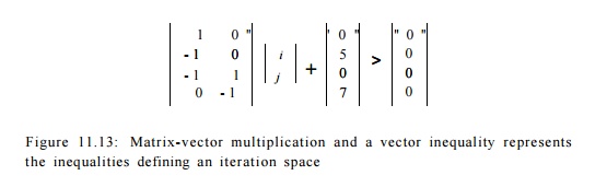
As another example, the inequality i < 5 is equivalent to (—l)i + (0)j+5 > 0, and is represented by the second row of B and b in Fig.  11.13.  Also, j > i becomes ( — + + 0 > 0 and is represented by the third row.  Finally, j < 7 becomes (0)i + + 7 > 0 and is the last row of the matrix and vector.

Manipulating Inequalities

To convert inequalities, as in Example 11.8, we can perform transforma-tions much as we do for equalities, e.g., adding or subtracting from both sides, or multiplying both sides by a constant. The only special rule we must remember is that when we multiply both sides by a negative number, we have to reverse the direction of the inequality. Thus, i < 5, multiplied by — 1, becomes —i > —5. Adding 5 to both sides, gives — i + 5 > 0, which is essentially the second row of Fig. 11.13.

4. Incorporating Symbolic Constants

Sometimes, we need to optimize a loop nest that involves certain variables that are loop-invariant for all the loops in the nest. We call such variables symbolic constants, but to describe the boundaries of an iteration space we need to treat them as variables and create an entry for them in the vector of loop indexes, i.e., the vector i in the general formulation of inequalities (11.1).

Example 11.9 :  Consider the simple loop:

 for (i=0; i <= n; i++)  {

 }     

This loop defines a one-dimensional iteration space, with index i, bounded by i  > 0 and i < n. Since n is a symbolic constant, we need to include it as a variable, giving us a vector of loop indexes [i,n]. In matrix-vector form, this iteration space is defined by

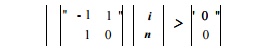
Notice that, although the vector of array indexes has two dimensions, only the first of these, representing i, is part of the output — the set of points lying with the iteration space. •

5. Controlling the Order of Execution

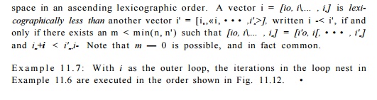
The linear inequalities extracted from the lower and upper bounds of a loop body define a set of iterations over a convex polyhedron. As such, the represen-tation assumes no execution ordering between iterations within the iteration space. The original program imposes one sequential order on the iterations, which is the lexicographic order with respect to the loop index variables ordered from the outermost to the innermost. However, the iterations in the space can be executed in any order as long as their data dependences are honored (i.e., the order in which writes and reads of any array element are performed by the various assignment statements inside the loop nest do not change).

The problem of how we choose an ordering that honors the data dependences and optimizes for data locality and parallelism is hard and is dealt with later starting from Section 11.7. Here we assume that a legal and desirable ordering is given, and show how to generate code that enforce the ordering. Let us start by showing an alternative ordering for Example 11.6.

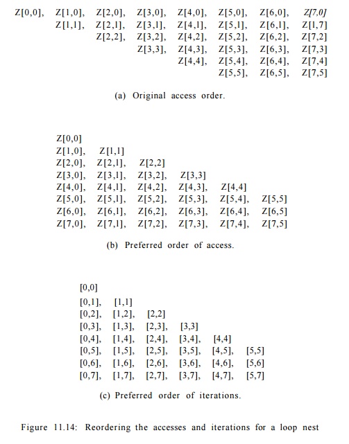
Example 11.10 : There are no dependences between iterations in the program in Example  11.6. We can therefore execute the iterations in arbitrary order, sequentially or concurrently.  Since iteration accesses element Z[j, i]  in the code, the original program visits the array in the order of Fig. 11.14(a). To improve spatial locality, we prefer to visit contiguous words in the array consecutively, as in Fig. 11.14(b).

This access pattern is obtained if we execute the iterations in the order shown in Fig. 11.14(c). That is, instead of sweeping the iteration space in Fig. 11.11 horizontally, we sweep the iteration space vertically, so j becomes the index of the outer loop. The code that executes the iterations in the above order is

Given a convex polyhedron and an ordering of the index variables, how do we generate the loop bounds that sweep through the space in lexicographic order of the variables? In the example above, the constraint i < j shows up as a lower bound for index j in the inner loop in the original program, but as an upper bound for index «, again in the inner loop, in the transformed program.

The bounds of the outermost loop, expressed as linear combinations of sym-bolic constants and constants, define the range of all the possible values it can take on. The bounds for inner loop variables are expressed as linear combi-nations of outer loop index variables, symbolic constants and constants. They define the range the variable can take on for each combination of values in outer loop variables.

Projection

Geometrically speaking, we can find the loop bounds of the outer loop index in a two-deep loop nest by projecting the convex polyhedron representing the iteration space onto the outer dimension of the space. The projection of a polyhedron on a lower-dimensional space is intuitively the shadow cast by the object onto that space. The projection of the two-dimensional iteration space in Fig. 11.11 opto the i axis is the vertical line from 0 to 5; and the projection onto

the j axis is the horizontal line from 0 to 7. When we project a 3-dimensional object along the z axis onto a 2-dimensional x and y plane, we eliminate variable z, losing the height of the individual points and simply record the 2-dimensional footprint of the object in the x-y plane.

Loop bound generation is only one of the many uses of projection.  Projection can be  defined formally as follows. Let S be an n-dimensional polyhedron.

The  projection  of S  onto the  first m  of its dimensions is  the set  of points (xi,x2,...   ,xm) such that  for some x m  +  1  , x m  +  2  , •••   ,xn, vector [xi,x2,...   ,xn] is  in  S. We  can compute projection using Fourier-Motzkin  elimination,  as follows:        

Algorithm 11.11 : Fourier-Motzkin elimination. 

INPUT : A polyhedron S with variables linear constraints involving the variables X{. to be the variable to be eliminated.

That is, 5 is a set of One given variable xm is specified

OUTPUT : A polyhedron 5" with variables x1,... ,xm-1,xm+i,... ,xn (i.e., all the variables of S except for xm) that is the projection of S onto dimensions other than the mth .

METHOD : Let C be all the constraints in S involving xm.  Do the following:

1. For every pair of a lower bound and an upper bound on xm    in C, such as

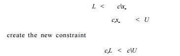
Note that c1  and c₂    are integers, but L and U may be expressions with

variables  other  than  x_m.

2.          If integers c1 and c₂ have a common factor, divide both sides by that factor.

3. If the new constraint is not satisfiable, then there is no solution to S; i.e.,  the polyhedra 5 and S' are both empty spaces.

4. S'  is the set of constraints S - C,  plus all the constraints generated in  step 2.  

Note, incidentally, that if x_m has u lower bounds and v upper bounds, elimi-nating x_m produces up to uv inequalities, but no more. •

The constraints added in step (1) of Algorithm 11.11 correspond to the im-plications of constraints C on the remaining variables in the system. Therefore, there is a solution in S' if and only if there exists at least one corresponding solution in S.  Given a solution in S' the range of the  corresponding xm    can be found by replacing all variables but xm in the constraints C by their actual values.

Example 11.12 : Consider the inequalities defining the iteration space in Fig. 11.11. Suppose we wish to use Fourier-Motzkin elimination to project the two-dimensional space away from the i dimension and onto the j dimension. There is one lower bound on i: 0 < i and two upper bounds: i < j and i < 5. This generates two constraints: 0 < j and 0 < 5. The latter is trivially true and can be ignored. The former gives the lower bound on j, and the original upper bound j < 7 gives the upper bound. •

Loop - Bounds  Generation

Now that we have defined Fourier-Motzkin elimination, the algorithm to gen-erate the loop bounds to iterate over a convex polyhedron (Algorithm 11.13) is straightforward. We compute the loop bounds in order, from the innermost to the outer loops. All the inequalities involving the innermost loop index vari-ables are written as the variable's lower or upper bounds. We then project away the dimension representing the innermost loop and obtain a polyhedron with one fewer dimension. We repeat until the bounds for all the loop index variables are found.

Algorithm 11.13 : Computing bounds for a given order of variables.

INPUT :  A convex polyhedron  S over variables v1,...  ,vn.

OUTPUT : A set of lower bounds L{ and upper bounds Ui for each vi, expressed only in terms of the fj's, for j < i.

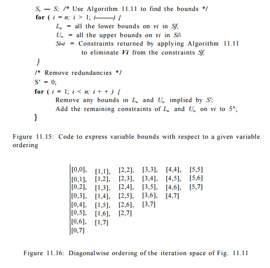
METHOD : The algorithm is described in Fig. 11.15.

Example 1 1 . 1 4 :  We apply Algorithm 11.13 to generate the loop bounds that sweep the the iteration space of Fig. 11.11 vertically. The variables are ordered j, i. The algorithm generates these bounds:

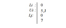
We need to satisfy all the constraints, thus the bound on i is min(5, j). There are no redundancies in this example.

6. Changing Axes

Note that sweeping the iteration space horizontally and vertically, as discussed above, are just two of the most common ways of visiting the iteration space. There are many other possibilities; for example, we can sweep the iteration space in Example 11.6 diagonal by diagonal, as discussed below in Example 11.15.

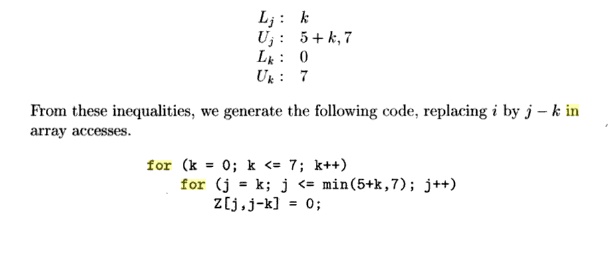
Example 1 1 . 1 5 : We can sweep the iteration space shown in Fig. 11.11 diag-onally using the order shown in Fig. 11.16. The difference between the coordi-nates j and i in each diagonal is a constant, starting with 0 and ending with 7. Thus, we define a new variable k = j — i and sweep through the iteration space in lexicographic order with respect to k and j. Substituting i = j — k in the inequalities we get:

To create the loop bounds for the order described above, we can apply Algo-rithm 11.13 to the above set of inequalities with variable ordering k, j.

In general, we can change the axes of a polyhedron by creating new loop index variables that represent affine combinations of the original variables, and defining an ordering on those variables. The hard problem lies in choosing the right axes to satisfy the data dependences while achieving the parallelism and locality objectives. We discuss this problem starting with Section 11.7. What we have established here is that once the axes are chosen, it is straightforward to generate the desired code, as shown in Example 11.15.

There are many other iteration-traversal orders not handled by this tech-nique. For example, we may wish to visit all the odd rows in an iteration space before we visit the even rows. Or, we may want to start with the iterations in the middle of the iteration space and progress to the fringes. For applications that have affine access functions, however, the techniques described here cover most of the desirable iteration orderings.

7. Exercises for Section 11.3

Exercise 11. 3. 1 : Convert each of the following loops to a form where the loop indexes are each incremented by 1:

a ) f o r (i=10; i<50;  i = i + 7 ) X [ i , i + 1 ] = 0 ; .

b) f o r (i=  - 3 ; i<=10; i=i+2)  X[i] = x [ i + l ] ; .

c) f o r (i=50; i>=10; i — ) X[i]  = 0; .

Exercise 11. 3 . 2 : Draw or describe the iteration spaces for each of the follow-ing loop nests:

a) The loop nest of Fig. 11.17(a).

b) The loop nest of Fig. 11.17(b).

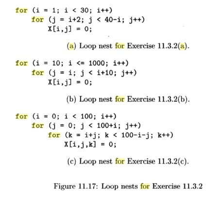
c)  The loop nest of Fig. 11.17(c).

Exercise 11 . 3 . 3: Write the constraints implied by each of the loop nests of Fig. 11.17 in the form of (11.1). That is, give the values of the vectors i and b and the matrix B.

Exercise 1 1 . 3 . 4 :  Reverse each of the loop-nesting orders for the nests of Fig.

11.17.

Exercise 11.3.5 : Use the Fourier-Motzkin elimination algorithm to eliminate i from each of the sets of constraints obtained in Exercise 11.3.3.

Exercise 11 . 3 . 6: Use the Fourier-Motzkin elimination algorithm to eliminate j from each of the sets of constraints obtained in Exercise 11.3.3.

Exercise 1 1 . 3 . 7 : For each of the loop nests in Fig. 11.17, rewrite the code so the axis i is replaced by the major diagonal, i.e., the direction of the axis is characterized by i = j. The new axis should correspond to the outermost loop.

Exercise 11 . 3 . 8:  Repeat Exercise 11.3.7 for the following changes of axes:

a) Replace i by i + j; i.e., the direction of the axis is the lines for which i+j is a constant. The new axis corresponds to the outermost loop.

b)  Replace j by i — 2j.  The new axis corresponds to the outermost loop.

Exercise 11 . 3 . 9: Let A, B, and C be integer constants in the following loop, with C > 1 and B > A:

f o r  ( i  = A;  i  <=  B;  i  =  i  +  C)

Z [ i ] =  0;

Rewrite the loop so the incrementation of the loop variable is 1 and the initial-ization is to 0, that is, to be of the form

f o r  (j  = 0; j <=  D; j++)

Z[E*j + F] = 0 ;

for integers D, E, and F.  Express D, E, and F in terms of A, B, and C.

Exercise 11 . 3 . 10: For a generic two-loop nest

f o r  ( i  = 0; i  <=  A; i++)

f o r ( j = B*i+C; j  <=  D*i+E;

with A through E integer constants, write the constraints that define the loop nest's iteration space in matrix-vector form, i.e., in the form Bi + b = 0.

Exercise 1 1 . 3 . 1 1 : Repeat Exercise 11.3.10 for a generic two-loop nest with symbolic integer constants rn and n as in

f o r ( i = 0; i <= m; i++)

 f o r ( j = A*i+B; j  <= O i + n ; j++)

As before, A, B: and C stand for specific integer constants.  Only i, j, m, and n should be mentioned in the vector of unknowns. Also, remember that only i and j are output variables for the expression.