Data Reuse

Data Reuse

1 Types of Reuse

2 Self Reuse

3 Self-Spatial Reuse

4 Group Reuse

5 Exercises for Section 11.5

From array access functions we derive two kinds of information useful for locality optimization and parallelization:

1.         Data reuse: for locality optimization, we wish to identify sets of iterations that access the same data or the same cache line.

2.         Data dependence: for correctness of parallelization and locality loop trans-formations, we wish to identify all the data dependences in the code. Re-call that two (not necessarily distinct) accesses have a data dependence if instances of the accesses may refer to the same memory location, and at least one of them is a write.

In many cases, whenever we identify iterations that reuse the same data, there are data dependences between them.

Whenever there is a data dependence, obviously the same data is reused. For example, in matrix multiplication, the same element in the output array is written 0(n) times. The write operations must be executed in the original execution order;³ there is reuse because we can allocate the same element to a register.

However, not all reuse can be exploited in locality optimizations; here is an example illustrating this issue.

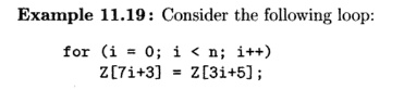
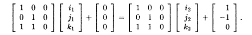
We observe that the loop writes to a different location at each iteration, so there are no reuses or dependences on the different write operations. The loop, how-ever, reads locations 5 , 8 , 1 1 , 1 4 , 1 7 , . . . , and writes locations 3 , 1 0 , 1 7 , 2 4 , — The read and write iterations access the same elements 17, 38, and 59 and so on. That is, the integers of the form 17 + 21 j for j = 0,1, 2 , . . . are all those integers that can be written both as 7ii  = 3 and as 3i2   + 5, for some integers i1 and i 2 .  However, this reuse occurs rarely, and cannot be exploited easily if at all.

Data dependence is different from reuse analysis in that one of the accesses sharing a data dependence must be a write access. More importantly, data de-pendence needs to be both correct and precise. It needs to find all dependences for correctness, and it should not find spurious dependences because they can cause unnecessary serialization.

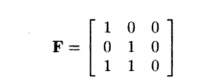
With data reuse, we only need to find where most of the exploitable reuses are. This problem is much simpler, so we take up this topic here in this section and tackle data dependences in the next. We simplify reuse analysis by ignoring loop bounds, because they seldom change the shape of the reuse. Much of the reuse exploitable by affine partitioning resides among instances of the same array accesses, and accesses that share the same coefficient matrix (what we have typically called F in the affine index function). As shown above, access patterns like 7% + 3 and 3i + 5 have no reuse of interest.

1. Types of Reuse

We first start with Example 11.20 to illustrate the different kinds of data reuses. In the following, we need to distinguish between the access as an instruction in a program, e.g., x  = Z [ i , j ] , from the execution of this instruction many times, as we execute the loop nest.  For emphasis, we may refer to the statement itself as a static  access,  while the various iterations of the statement as we execute its loop nest  are called dynamic  accesses.

Reuses can be classified as self versus group. If iterations reusing the same data come from the same static access, we refer to the reuse as self reuse; if they come from different accesses, we refer to it as group reuse. The reuse is temporal if the same exact location is referenced; it is spatial if the same cache line is referenced.

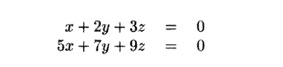
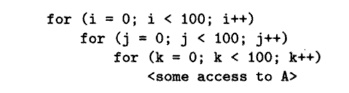
Example 11.20 :  Consider the following loop nest:

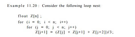
Accesses Z[j], Z[j + 1], and Z[j + 2] each have self-spatial reuse because con-secutive iterations of the same access refer to contiguous array elements. Pre-sumably contiguous elements are very likely to reside on the same cache line. In addition, they all have self-temporal reuse, since the exact elements are used over and over again in each iteration in the outer loop. In addition, they all have the same coefficient matrix, and thus have group reuse. There is group reuse, both temporal and spatial, between the different accesses.  Although there are 4 n 2 accesses in this code, if the reuse can be exploited, we only need to bring in about n / c cache lines into the cache, where c is the number of words in a cache line.  We drop a factor of n due to self-spatial reuse, a factor of c to due to spatial locality, and finally a factor of 4 due to group reuse.

In the following, we show how we can use linear algebra to extract the reuse information from affine array accesses. We are interested in not just finding how much potential savings there are, but also which iterations are reusing the data so that we can try to move them close together to exploit the reuse.

2. Self Reuse

There can be substantial savings in memory accesses by exploiting self reuse. If the data referenced by a static access has k dimensions and the access is nested in a loop d deep, for some d > k, then the same data can be reused n^d~^k times, where n is the number of iterations in each loop. For example, if a 3-deep loop nest accesses one column of an array, then there is a potential savings factor of n2    accesses. It turns out that the dimensionality of an access corresponds to the concept of the  rank of the coefficient matrix in the access, and we can find which iterations refer to the same location by finding the null space of the matrix, as explained below.

Rank of a Matrix

The rank of a matrix F is the largest number of columns (or equivalently, rows) of F that are linearly independent. A set of vectors is linearly independent if none of the vectors can be written as a linear combination of finitely many other vectors in the set.

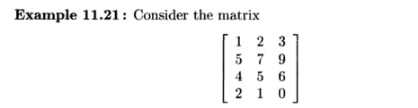
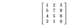
Notice that the second row is the sum of the first and third rows, while the fourth row is the third row minus twice the first row. However, the first and third rows are linearly independent; neither is a multiple of the other. Thus, the rank of the matrix is 2.

We could also draw this conclusion by examining the columns. The third column is twice the second column minus the first column. On the other hand, any two columns are linearly independent. Again, we conclude that the rank is 2.

Example 1 1 . 2 2 : Let us look at the array accesses in Fig. 11.18. The first access, X[i — 1], has dimension 1, because the rank of the matrix [1 0] is 1. That is, the one row is linearly independent, as is the first column.

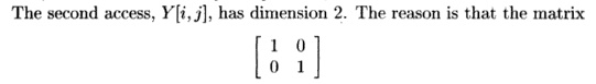
has two independent rows (and therefore two independent columns, of course). The third access, Y[j, j + 1], is of dimension 1, because the matrix

has rank 1. Note that the two rows are identical, so only one is linearly in-dependent. Equivalently, the first column is 0 times the second column, so the columns are not independent. Intuitively, in a large, square array Y, the only elements accessed lie along a one-dimensional line, just above the main diagonal.

The fourth access, Y[l,2] has dimension 0, because a matrix of all 0's has rank 0. Note that for such a matrix, we cannot find a linear sum of even one row that is nonzero. Finally, the last access, Z[i,i,2 * i + j], has dimension 2. Note that in the matrix for this access

the last two rows are linearly independent; neither is a multiple of the other.

However, the first row is a linear "sum" of the other two rows, with both coefficients 0.

Null Space of a Matrix

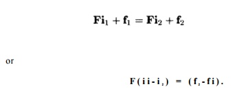
A reference in a d-deep loop nest with rank r accesses 0(nr) data elements in 0(nd) iterations, so on average, 0(nd~r) iterations must refer to the same array element. Which iterations access the same data? Suppose an access in this loop nest is represented by matrix-vector combination F and f. Let i and i' be two iterations that refer to the same array element. Then Fi + f = Fi' + f.

Rearranging terms, we get 

There is a well-known concept from linear algebra that characterizes when i and i' satisfy the above equation. The set of all solutions to the equation Fv = 0 is called the null space of F. Thus, two iterations refer to the same array element if the difference of their loop-index vectors belongs to the null space of matrix F.

It is easy to see that the null vector, v = 0, always satisfies Fv = 0. That is, two iterations surely refer to the same array element if their difference is 0; in other words, if they are really the same iteration. Also, the null space is truly a vector space. That is, if F v i = 0 and F v 2 = 0, then F(vi + v 2 ) = 0 and F(cvi) = 0.

If the matrix F is fully ranked, that is, its rank is d, then the null space of F consists of only the null vector. In that case, iterations in a loop nest all refer to different data. In general, the dimension of the null space, also known as the nullity, is d — r. If d > r, then for each element there is a (d — r)-dimensional space of iterations that access that element.

The null space can be represented by its basis vectors. A ^-dimensional null space is represented by k independent vectors; any vector that can be expressed as a linear combination of the basis vectors belongs to the null space.

Example 11 . 23 :  Let us reconsider the matrix of Example 11.21:

We determined in that example that the rank of the matrix is 2; thus the nullity is 3 - 2 = 1. To find a basis for the null space, which in this case must be a single nonzero vector of length 3, we may suppose a vector in the null space to be  [x,y,z]  and try to solve the equation

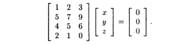
If we multiply the first two rows by the vector of unknowns, we get the two equations

We could write the equations that come from the third and fourth rows as well, but because there are no three linearly independent rows, we know that the additional equations add no new constraints on x, y, and z. For instance, the equation we get from the third row, Ax + 5y + Qz = 0 can be obtained by subtracting the first equation from the second.

We must eliminate as many variables as we can from the above equations. Start by using the first equation to solve for x; that is, x — —2y — 3z. Then substitute for x in the second equation, to get — 3y = 6z, or y = —2z. Since x = —2y — 3z, and y = —2z:  it follows that x = z. Thus, the vector [x,y,z] is really [z, —2z,z]. We may pick any nonzero value of z to form the one and only basis vector for the null space. For example, we may choose z = 1 and use [1, —2,1] as the basis of the null space.

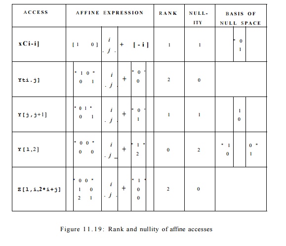
Example 1 1 . 2 4 : The rank, nullity, and null space for each of the references in Example 11.17 are shown in Fig. 11.19. Observe that the sum of the rank and nullity in all the cases is the depth of the loop nest, 2. Since the accesses

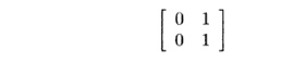
and Z[l, i, 2 * i + j] have a rank of 2, all iterations refer to different locations. Accesses X[i — 1] and Y[j, j +   both have rank-1 matrices, so 0(n) iterations refer to the same location.  In the former case, entire rows in the iteration space refer to the same location.  In other words, iterations that differ only in the j dimension share the same location, which is succinctly represented by the basis of the null space, [0,1].  For Y[j,j + 1],  entire columns in the iteration space refer to the same location, and this fact is succinctly represented by the basis of the null space, [1,0].

Finally, the access F[l,2] refers to the same location in all the iterations. The null space corresponding has 2 basis vectors, [0,1], [1,0], meaning that all pairs of iterations in the loop nest refer to exactly the same location. •

3. Self-Spatial Reuse

The analysis of spatial reuse depends on the data layout of the matrix. C matrices are laid out in row-major order and Fortran matrices are laid out in column-major order. In other words, array elements X[iJ] and X[i,j + 1] are

contiguous in C and X[i, j] and X[i + 1, j] are contiguous in Fortran. Without loss of generality, in the rest of the chapter, we shall adopt the C (row-major) array layout.

As a first approximation, we consider two array elements to share the same cache line if and only if they share the same row in a two-dimensional array. More generally, in an array of d dimensions, we take array elements to share a cache line if they differ only in the last dimension. Since for a typical array and cache, many array elements can fit in one cache line, there is significant speedup to be had by accessing an entire row in order, even though, strictly speaking, we occasionally have to wait to load a new cache line.

The trick to discovering and taking advantage of self-spatial reuse is to drop the last row from the coefficient matrix F. If the resulting truncated matrix has rank that is less than the depth of the loop nest, then we can assure spatial locality by making sure that the innermost loop varies only the last coordinate of the array.

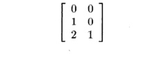
Example  1 1 . 2 5 :  Consider the last access,  Z[l, i,2* i+ j], in Fig.  1 1 . 1 9 .  If we delete the last row, we are left with the truncated matrix

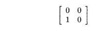
The rank of this matrix is evidently 1, and since the loop nest has depth 2, there is the opportunity for spatial reuse. In this case, since j is the inner-loop index, the inner loop visits contiguous elements of the array Z stored in row-major order. Making i the inner-loop index will not yield spatial locality, since as i changes, both the second and third dimensions change. •

The general rule for determining whether there is self-spatial reuse is as follows. As always, we assume that the loop indexes correspond to columns of the coefficient matrix in order, with the outermost loop first, and the innermost loop last. Then in order for there to be spatial reuse, the vector [ 0 , 0 , . . . , 0,1] must be in the null space of the truncated matrix. The reason is that if this vector is in the null space, then when we fix all loop indexes but the innermost one, we know that all dynamic accesses during one run through the inner loop vary in only the last array index. If the array is stored in row-major order, then these elements are all near one another, perhaps in the same cache line.

Example 11 . 26 : Note that [0,1] (transposed as a column vector) is in the null space of the truncated matrix of Example 11.25. Thus, as mentioned there, we expect that with j as the inner-loop index, there will be spatial locality. On the other hand, if we reverse the order of the loops, so i is the inner loop, then the coefficient matrix becomes 

Now,  [0,1] is not in the null space of this matrix. Rather, the null space is generated by the basis vector [1,0]. Thus, as we suggested in Example 11.25, we do not expect spatial locality if i is the inner loop.

We should observe, however, that the test for [ 0 , 0 , . . . , 0,1] being in the null space is not quite sufficient to assure spatial locality. For instance, suppose the  access  were  not  Z[l,i,2*i  + j]  but  Z[l,i,2*i  +  50*j]. Then, only  every fiftieth element of Z would be accessed during one run of the inner loop, and we would not reuse a cache line unless it were long enough to hold more than 50 elements.

4. Group Reuse

We compute group reuse only among accesses in a loop sharing the same coef-ficient matrix. Given two dynamic accesses Fii + fi and F i ₂ + f₂, reuse of the same data requires that

Suppose v is one solution to this equation. Then if w is any vector in the null space of F i , w + v is also a solution, and in fact those are all the solutions to the equation.

has two array accesses, Z[i,j] and Z[i — l,j]. Observe that these two accesses are both characterized by the coefficient matrix

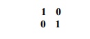
like the second access, Y"[i, j] in Fig. 11.19. This matrix has rank 2, so there is no self-temporal reuse.

However, each access exhibits self-spatial reuse. As described in Section 11.5.3, when we delete the bottom row of the matrix, we are left with only the top row, [1,0], which has rank 1. Since [0,1] is in the null space of this truncated matrix, we expect spatial reuse. As each incrementation of inner-loop index j increases the second array index by one, we in fact do access adjacent array elements, and will make maximum use of each cache line.

Although there is no self-temporal reuse for either access, observe that the two references Z[i,j] and Z[i — l,j] access almost the same set of array elements. That is, there is group-temporal reuse because the data read by access Z[i — l,j) is the same as the data written by access Z[i,j], except for the case i = 1. This simple pattern applies to the entire iteration space and can be exploited to improve data locality in the code. Formally, discounting the loop bounds, the two accesses  Z[i,j]  and  Z[i- l,j]  refer to the same location in iterations  (k,ji) and (%2, j 2 ) , respectively, provided

That is, ji = J2 and i2   = k + 1.

Notice that the reuse occurs along the i-axis the of the iteration space. That is, inner iteration (kih) occurs n iterations (of the loop) after the iteration

Thus, many iterations are executed before the data written is reused.

This data may or may not still be in the cache.  If the cache manages to hold two consecutive rows of matrix Z, then access Z[i — does not miss in the cache, and the total number of cache misses for the entire loop nest is n 2 / c , where c is the number of elements per cache line. Otherwise, there will be twice as many misses, since both static accesses require a new cache line for each c dynamic accesses.

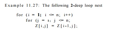
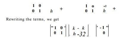
Example 11 . 28 :  Suppose there are two accesses

in a 3-deep loop nest, with indexes i, j, and k, from the outer to the inner loop. Then two accesses ii = [i1,ji,k1] and i₂ = [^2,^2,^2] reuse the same element whenever

One solution to this equation for a vector v = [i1 — i 2 , ji — j 2 , &i — &2] is v = [1, —1,0]; that is, i1 22 + 1, Ji = ji — 1, and k1 = &2 .4 However, the null space of the matrix   

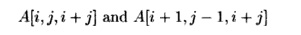
is generated by the basis vector [0,0,1]; that is, the third loop index, k, can be arbitrary. Thus, v, the solution to the above equation, is any vector [1, — l , m ] for some m.  Put another way, a dynamic access to A[i,j,i + j], in a loop nest with indexes i, j, and is reused not only by other dynamic accesses A[i, j, i+j] with the same values of i and j and a different value of k, but also by dynamic accesses A[i + 1, j — 1, i + j] with loop index values i + 1, j — 1, and any value of k.

Although we shall not do so here, we can reason about group-spatial reuse analogously. As per the discussion of self-spatial reuse, we simply drop the last dimension from consideration.

The extent of reuse is different for the different categories of reuse. Self-temporal reuse gives the most benefit: a reference with a ^-dimensional null space reuses the same data 0(n^k) times. The extent of self-spatial reuse is limited by the length of the cache line. Finally, the extent of group reuse is limited by the number of references in a group sharing the reuse.

5. Exercises for Section 11.5

Exercise 1 1 . 5 . 1 : Compute the ranks of each of the matrices in Fig. 11.20. Give both a maximal set of linearly dependent columns and a maximal set of linearly dependent rows. 

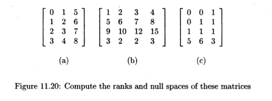
Exercise 11.5.2 : Find a basis for the null space of each matrix in Fig. 11.20.

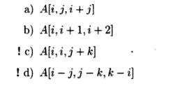
Exercise 11 . 5 . 3: Assume that the iteration space has dimensions (variables) i, j, and k. For each of the accesses below, describe the subspaces that refer to the following single elements of the array:

Exercise 11 . 5 . 4: Suppose array A is stored in row-major order and accessed inside the following loop nest:

Indicate for each of the following accesses whether it is possible to rewrite the loops so that the access to A exhibits self-spatial reuse; that is, entire cache lines are used consecutively. Show how to rewrite the loops, if so. Note: the rewriting of the loops may involve both reordering and introduction of new loop indexes. However, you may not change the layout of the array, e.g., by changing it to column-major order. Also note: in general, reordering of loop indexes may be legal or illegal, depending on criteria we develop in the next section. However, in this case, where the effect of each access is simply to set an array element to 0, you do not have to worry about the effect of reordering loops as far as the semantics of the program is concerned.

Exercise 1 1 . 5 . 5 : In Section 11.5.3 we commented that we get spatial locality  if the innermost loop varies only as the last coordinate of an array access.  However, that assertion depended on our assumption that the array was stored  in row-major order. What condition would assure spatial locality if the array  were stored in column-major order? 

 Exercise 1 1 . 5 . 6 : In Example 11.28 we observed that the the existence of reuse  between two similar accesses depended heavily on the particular expressions for  the coordinates of the array. Generalize our observation there to determine  for which functions f(i,j) there is reuse between the accesses A[i,j,i + j] and  A[i + l,j-l,f(iJ)}. 

 Exercise 1 1 . 5 . 7 : In Example 11.27 we suggested that there will be more cache  misses than necessary if rows of the matrix Z are so long that they do not fit in the cache. If that is the case, how could you rewrite the loop nest in order to Guarantee group-spatial reuse?