Basic Concepts of Optimizing for Parallelism and Locality

Basic Concepts

1 Multiprocessors

2 Parallelism in Applications

3 Loop-Level Parallelism

4 Data Locality

5 Introduction to Affine Transform Theory

This section introduces the basic concepts related to parallelization and local-ity optimization. If operations can be executed in parallel, they also can be reordered for other goals such as locality. Conversely, if data dependences in a program dictate that instructions in a program must execute serially, there is obviously no parallelism, nor is there any opportunity to reorder instruc-tions to improve locality. Thus parallelization analysis also finds the available opportunities for code motion to improve data locality.

To minimize communication in parallel code, we group together all related operations and assign them to the same processor. The resulting code must therefore have data locality. One crude approach to getting good data locality on a uniprocessor is to have the processor execute the code assigned to each processor in succession.

In this introduction, we start by presenting an overview of parallel computer architectures. We then show the basic concepts in parallelization, the kind of transformations that can make a big difference, as well as the concepts useful for parallelization. We then discuss how similar considerations can be used to optimize locality. Finally, we introduce informally the mathematical concepts used in this chapter.

1. Multiprocessors

The most popular parallel machine architecture is the symmetric multiproces-sor (SMP). High-performance personal computers often have two processors, and many server machines have four, eight, and some even tens of processors. Moreover, as it has become feasible for several high-performance processors to fit on a single chip, multiprocessors have become even more widely used.

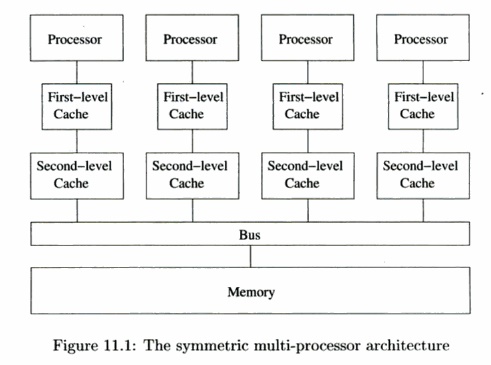
Processors on a symmetric multiprocessor share the same address space. To communicate, a processor can simply write to a memory location, which is then read by any other processor. Symmetric multiprocessors are so named because all processors can access all of the memory in the system with a uniform access time. Fig. 11.1 shows the high-level architecture of a multiprocessor. The processors may have their own first-level, second-level, and in some cases, even a third-level cache. The highest-level caches are connected to physical memory through typically a shared bus.

Symmetric multiprocessors use a coherent cache protocol to hide the presence of caches from the programmer.  Under such a protocol, several processors are allowed to keep copies of the same cache line1 at the same time, provided that they are only reading the data. When a processor wishes to write to a cache line, copies from all other caches are removed. When a processor requests data not found in its cache, the request goes out on the shared bus, and the data will be fetched either from memory or from the cache of another processor.

The time taken for one processor to communicate with another is about twice the cost of a memory access. The data, in units of cache lines, must first be written from the first processor's cache to memory, and then fetched from the memory to the cache of the second processor. You may think that interprocessor communication is relatively cheap, since it is only about twice as slow as a memory access. However, you must remember that memory accesses are very expensive when compared to cache hits—they can be a hundred times slower. This analysis brings home the similarity between efficient parallelization and locality analysis. For a processor to perform well, either on its own or in the context of a multiprocessor, it must find most of the data it operates on in its cache.

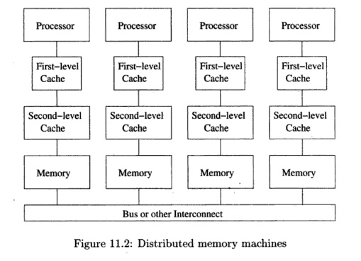
In the early 2000's, the design of symmetric multiprocessors no longer scaled beyond tens of processors, because the shared bus, or any other kind of inter-connect for that matter, could not operate at speed with the increasing number of processors. To make processor designs scalable, architects introduced yet an-other level in the memory hierarchy. Instead of having memory that is equally far away for each processor, they distributed the memories so that each pro-cessor could access its local memory quickly as shown in Fig. 11.2. Remote memories thus constituted the next level of the memory hierarchy; they are collectively bigger but also take longer to access. Analogous to the principle in memory-hierarchy design that fast stores are necessarily small, machines that support fast interprocessor communication necessarily have a small number of processors.

There are two variants of a parallel machine with distributed memories: NUM A (nonuniform memory access) machines and message-passing machines. NUM A architectures provide a shared address space to the software, allowing processors to communicate by reading and writing shared memory. On message-passing machines, however, processors have disjoint address spaces, and proces-sors communicate by sending messages to each other. Note that even though it is simpler to write code for shared memory machines, the software must have good locality for either type of machine to perform well.

2. Parallelism in Applications

We use two high-level metrics to estimate how well a parallel application will perform: parallelism coverage which is the percentage of the computation that runs in parallel, granularity of parallelism, which is the amount of computation that each processor can execute without synchronizing or communicating with others. One particularly attractive target of parallelization is loops: a loop may have many iterations, and if they are independent of each other, we have found a great source of parallelism.

Amdahl's  Law

The significance of parallelism coverage is succinctly captured by Amdahl's Law.

Amdahl's  Law states that,  if / is the fraction of the code parallelized,  and if the parallelized version runs on a p-processor machine with no communication or parallelization overhead, the speedup is

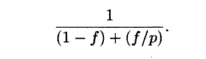
For example, if half of the computation remains sequential, the computation can only double in speed, regardless of how many processors we use. The speedup achievable is a factor of 1.6 if we have 4 processors. Even if the parallelism coverage is 90%, we get at most a factor of 3 speed up on 4 processors, and a factor of 10 on an unlimited number of processors.

Granularity  of Parallelism

It is ideal if the entire computation of an application can be partitioned into many independent coarse-grain tasks because we can simply assign the differ-ent tasks to different processors. One such example is the SETI (Search for Extra-Terrestrial Intelligence) project, which is an experiment that uses home computers connected over the Internet to analyze different portions of radio telescope data in parallel. Each unit of work, requiring only a small amount of input and generating a small amount of output, can be performed indepen-dently of all others. As a result, such a computation runs well on machines over the Internet, which has relatively high communication latency (delay) and low bandwidth.

Most applications require more communication and interaction between pro-cessors, yet still allow coarse-grained parallelism. Consider, for example, the web server responsible for serving a large number of mostly independent re-quests out of a common database. We can run the application on a multi-processor, with a thread implementing the database and a number of other threads servicing user requests. Other examples include drug design or airfoil simulation, where the results of many different parameters can be evaluated independently. Sometimes the evaluation of even just one set of parameters in a simulation takes so long that it is desirable to speed it up with paralleliza-tion. As the granularity of available parallelism in an application decreases, better interprocessor communication support and more programming effort are needed.

Many long-running scientific and engineering applications, with their simple control structures and large data sets, can be more readily parallelized at a finer grain than the applications mentioned above. Thus, this chapter is devoted pri-marily to techniques that apply to numerical applications, and in particular, to programs that spend most of their time manipulating data in multidimensional arrays. We shall examine this class of programs next.

3. Loop-Level Parallelism

Loops are the main target for parallelization, especially in applications using arrays. Long running applications tend to have large arrays, which lead to loops that have many iterations, One for each element in the array. It is not uncommon to find loops whose iterations are independent of one another. We can divide the large number of iterations of such loops among the processors. If the amount of work performed in each iteration is roughly the same, simply dividing the iterations evenly across processors will achieve maximum paral-lelism. Example 11.1 is an extremely simple example showing how we can take advantage of loop-level parallelism.

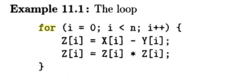
computes the square of diferences between elements in vectors X and Y and stores it into Z. The loop is parallelizable because each iteration accesses a different set of data. We can execute the loop on a computer with M processors by giving each processor an unique ID p = 0 , 1 , . . . , M - 1 and having each processor execute the same code:

Task-Level Parallelism

It is possible to find parallelism outside of iterations in a loop. For example, we can assign two different function invocations, or two independent loops, to two processors. This form of parallelism is known as task parallelism. The task level is not as attractive a source of parallelism as is the loop level. The reason is that the number of independent tasks is a constant for each program and does not scale with the size of the data, as does the number of iterations of a typical loop. Moreover, the tasks generally are not of equal size, so it is hard to keep all the processors busy all the time.

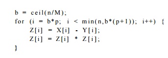
We divide the iterations in the loop evenly among the processors; the pth processor is given the pth swath of iterations to execute. Note that the number of iterations may not be divisible by M, so we assure that the last processor does not execute past the bound of the original loop by introducing a minimum operation. •

The parallel code shown in Example 11.1 is an SPMD (Single Program Multiple Data) program. The same code is executed by all processors, but it is parameterized by an identifier unique to each processor, so different proces-sors can take different actions. Typically one processor, known as the master, executes all the serial part of the computation. The master processor, upon

reaching a parallelized section of the code, wakes up all the  slave processors. All the processors execute the parallelized regions of the  code. At the end of each parallelized region of code, all the processors participate in a barrier synchronization. Any operation executed before a processor enters a synchro-nization barrier is guaranteed to be completed before any other processors are allowed to leave the barrier and execute operations that come after the barrier.

If we parallelize only little loops like those in Example 11.1, then the re-sulting code is likely to have low parallelism coverage and relatively fine-grain parallelism. We prefer to parallelize the outermost loops in a program, as that yields the coarsest granularity of parallelism. Consider, for example, the appli-cation of a two-dimensional FFT transformation that operates on an n x n data set.  Such a program performs n FFT's on the rows of the data, then another n FFT's on the columns.  It is preferable to assign each of the n independent FFT ' s to one processor each, rather than trying to use several processors to collaborate on one FFT . The code is easier to write, the parallelism coverage for the algorithm is 100%, and the code has good data locality as it requires no communication at all while computing an F F T .

Many applications do not have large outermost loops that are parallelizable. The execution time of these applications, however, is often dominated by time-consuming kernels, which may have hundreds of lines of code consisting of loops with different nesting levels. It is sometimes possible to take the kernel, reorganize its computation and partition it into mostly independent units by focusing on its locality.

4. Data Locality

There are two somewhat different notions of data locality that need to be con-sidered when parallelizing programs. Temporal locality occurs when the same data is used several times within a short time period. Spatial locality occurs when different data elements that are located near to each other are used within a short period of time. An important form of spatial locality occurs when all the elements that appear on one cache line are used together. The reason is that as soon as one element from a cache line is needed, all the elements in the same line are brought to the cache and will probably still be there if they are used soon. The effect of this spatial locality is that cache misses are minimized, with a resulting important speedup of the program.

Kernels can often be written in many semantically equivalent ways but with widely varying data localities and performances. Example 11.2 shows an alter-native way of expressing the computation in Example 11.1.

Example 11. 2 : Like Example 11.1 the following also finds the squares of differences between elements in vectors X and Y.

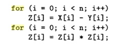
The first loop finds the differences, the second finds the squares. Code like this appears often in real programs, because that is how we can optimize a program for vector machines, which are supercomputers which have instructions that perform simple arithmetic operations on vectors at a time. We see that the bodies of the two loops here are fused as one in Example 11.1.

Given that the two programs perform the same computation, which performs better? The fused loop in Example 11.1 has better performance because it has better data locality. Each difference is squared immediately, as soon as it is produced; in fact, we can hold the difference in a register, square it, and write the result just once into the memory location Z[i]. In contrast, the code in Example 11.1 fetches Z[i] once, and writes it twice. Moreover, if the size of the array is larger than the cache, Z1i1 needs to be refetched from memory the second time it is used in this example. Thus, this code can run significantly slower.

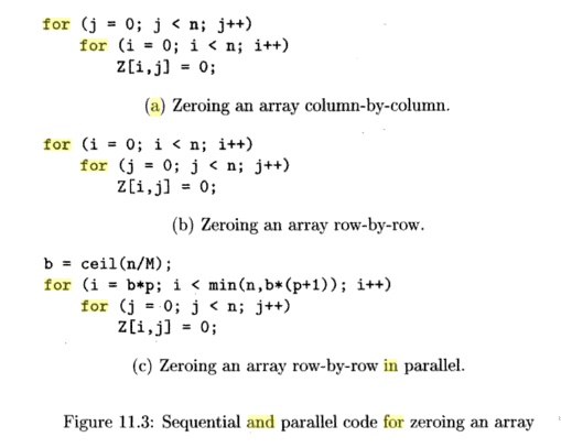
Example 11.3:  Suppose we want to set array Z,  stored in row-major order (recall Section 6.4.3),  to all zeros. Fig.  11.3(a)  and  (b)  sweeps through the  array column-by-column and row-by-row, respectively. We can transpose the loops in Fig. 11.3(a) to arrive at Fig. 11.3(b). In terms of spatial locality, it is preferable to zero out the array row-by-row since all the words in a cache line are zeroed consecutively. In the column-by-column approach, even though each cache line is reused by consecutive iterations of the outer loop, cache lines will be thrown out before reuse if the size of a colum is greater than the size of the cache. For best performance, we parallelize the outer loop of Fig. 11.3(b) in a manner similar to that used in Example 11.1.   •

The two examples above illustrate several important characteristics associ-ated with numeric applications operating on arrays:

•              Array code often has many parallelizable loops.

•              When loops have parallelism, their iterations can be executed in arbitrary

order; they can be reordered to improve data locality drastically.

•              As we create large units of parallel computation that are independent of each other, executing these serially tends to produce good data locality.

5. Introduction to Affine Transform Theory

Writing correct and efficient sequential programs is difficult; writing parallel programs that are correct and efficient is even harder. The level of difficulty increases as the granularity of parallelism exploited decreases. As we see above, programmers must pay attention to data locality to get high performance. Fur-thermore, the task of taking an existing sequential program and parallelizing it is extremely hard. It is hard to catch all the dependences in the program, es-pecially if it is not a program with which we are familiar. Debugging a parallel program is harder yet, because errors can be nondeterministic.

Ideally, a parallelizing compiler automatically translates ordinary sequential programs into efficient parallel programs and optimizes the locality of these programs. Unfortunately, compilers without high-level knowledge about the application, can only preserve the semantics of the original algorithm, which may not be amenable to parallelization. Furthermore, programmers may have made arbitrary choices that limit the program's parallelism.

Successes in parallelization and locality optimizations have been demon-strated for Fortran numeric applications that operate on arrays with affine accesses. Without pointers and pointer arithmetic, Fortran is easier to ana-lyze. Note that not all applications have affine accesses; most notably, many numeric applications operate on sparse matrices whose elements are accessed indirectly through another array. This chapter focuses on the parallelization and optimizations of kernels, consisting of mostly tens of lines.

As illustrated by Examples 11.2 and 11.3, parallelization and locality op-timization require that we reason about the different instances of a loop and their relations with each other. This situation is very different from data-flow analysis, where we combine information associated with all instances together.

For the problem of optimizing loops with array accesses, we use three kinds of spaces. Each space can be thought of as points on a grid of one or more dimensions.

1.          The iteration space is the set of the dynamic execution instances in a computation, that is, the set of combinations of values taken on by the loop indexes.

2.          The data space is the set of array elements accessed.

3.          The processor space is the set of processors in the system. Normally, these processors are assigned integer numbers or vectors of integers to distinguish among them.

Given as input are a sequential order in which the iterations are executed and affine  array-access functions  (e.g.,  X[iJ + 1])  that  specify  which  instances  in the iteration space access which elements in the data space.

The output of the optimization, again represented as affine functions, defines what each processor does and when. To specify what each processor does, we use an affine function to assign instances in the original iteration space to processors. To specify when, we use an affine function to map instances in the iteration space to a new ordering. The schedule is derived by analyzing the array-access functions for data dependences and reuse patterns.

The following example will illustrate the three spaces — iteration, data, and processor. It will also introduce informally the important concepts and issues that need to be addressed in using these spaces to parallelize code. The concepts each will be covered in detail in later sections.

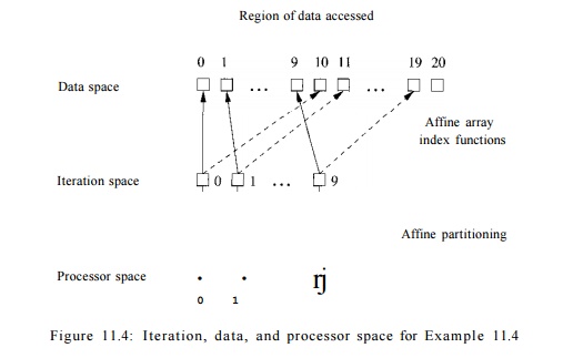
Example     11.4 :  Figure        11.4 illustrates the different spaces and their relations used in the following program:

float  Z[100]         ;

for     ( i      =  0;  i         <       10;  i++)

          Z[i+10]       =       Z [ i ] ;

The three spaces and the mappings among them are as follows:

1. Iteration Space: The iteration space is the  set of iterations,  whose ID's  are given by the values held by the loop index variables.  A d-deep loop  nest (i.e.,  d nested loops) has d index variables, and is thus modeled by   a G?-dimensional space.  The space of iterations is bounded by the lower  and upper bounds of the loop indexes.  The loop of this example defines a  one-dimensional space of 10 iterations, labeled by the loop index values:

 i = 0 , 1 , . . .  ,9 .    

2. Data Space: The data space is given directly by the array declarations.   In this example, elements in the array are indexed by a — 0 , 1 , . . . ,99.   Even though all arrays are linearized in a program's address space, we   treat n-dimensional arrays as n-dimensional spaces, and assume that the   individual indexes stay within their bounds.  In this example, the array is   one-dimensional anyway.   

3.  Processor Space: We pretend that there are an unbounded number of virtual processors in the system as our initial parallelization target. The processors are organized in a multidimensional space, one dimension for each loop in the nest we wish to parallelize. After parallelization, if we have fewer physical processors than virtual processors, we divide the vir-tual processors into even blocks, and assign a block each to a processor.

In this example, we need only ten processors, one for each iteration of the loop. We assume in Fig. 11.4 that processors are organized in a one-dimensional space and numbered 0 , 1 , . . . ,9, with loop iteration i assigned to processor i. If there were, say, only five processors, we could assign it-erations 0 and 1 to processor 0, iterations 2 and 3 to processor 1, and so on. Since iterations are independent, it doesn't matter how we do the assignment, as long as each of the five processors gets two iterations.

4.  Affine Array-Index Function: Each array access in the code specifies a mapping from an iteration in the iteration space to an array element in the data space. The access function is affine if it involves multiplying the loop index variables by constants and adding constants. Both the array index functions i + 10, and i are affine. From the access function, we can tell the dimension of the data accessed. In this case, since each index function has one loop variable, the space of accessed array elements is one dimensional.

5.   Affine Partitioning: We parallelize a loop by using an affine function to assign iterations in an iteration space to processors in the processor space. In our example, we simply assign iteration i to processor i. We can also specify a new execution order with affine functions. If we wish to execute the loop above sequentially, but in reverse, we can specify the ordering function succinctly with an affine expression 10 — i. Thus, iteration 9 is the 1st iteration to execute and so on.

6.  Region  of Data Accessed:  To find the best affine partitioning, it useful to know the region of data accessed by an iteration. We can get the region of data accessed by combining the iteration space information with the array index function. In this case, the array access Z[i + 10] touches the region {a | 10 < a < 20} and the access Z[i] touches the region {a10 < a < 10}.

7. Data Dependence: To determine if the loop is parallelizable, we ask if there is a data dependence that crosses the boundary of each iteration. For this example, we first consider the dependences of the write accesses in the loop. Since the access function Z[z + 10] maps different iterations to differ-ent array locations, there are no dependences regarding the order in which the various iterations write values to the array. Is there a dependence be-tween the read and write accesses? Since only Z[10], Z[ll],... , Z[19] are written (by the access Z[i + 10]), and only Z[0], Z[l],... , Z[9] are read (by the access Z[i]), there can be no dependencies regarding the relative order of a read and a write. Therefore, this loop is parallelizable. That is, each iteration of the loop is independent of all other iterations, and we can execute the iterations in parallel, or in any order we choose. Notice, however, that if we made a small change, say by increasing the upper limit on loop index i to 10 or more, then there would be dependencies, as some elements of array Z would be written on one iteration and then read 10 iterations later. In that case, the loop could not be parallelized completely, and we would have to think carefully about how iterations were partitioned among processors and how we ordered iterations.

Formulating the problem in terms of multidimensional spaces and affine mappings between these spaces lets us use standard mathematical techniques to solve the parallelization and locality optimization problem generally. For example, the region of data accessed can be found by the elimination of variables using the Fourier-Motzkin elimination algorithm. Data dependence is shown to be equivalent to the problem of integer linear programming. Finally, finding the affine partitioning corresponds to solving a set of linear constraints. Don't worry if you are not familiar with these concepts, as they will be explained starting in Section 11.3.