Summary

Summary

·           A variable which can assume finite number of possible values or an infinite sequence of countable real numbers is called a discrete random variable.

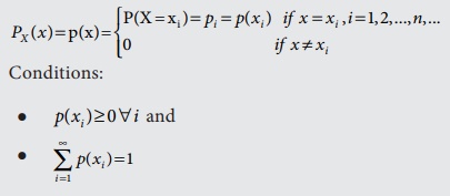
·           Probability mass function (p.m.f.)

·           Discrete distribution function (d.f.):

FX ( x) = P ( X ≤ x ) for all x ∈R

i .e., FX (x) = ∑ _{xi ≤ x} p(xi )

·           A random variable X which can take on any value (integral as well as fraction) in the interval is called continuous random variable.

·           Probability density function (p.d.f.)

The probability that a random variable X takes a value in the (open or closed) interval [t₁ ,t ₂ ] is given by the integral of a function called the probability density function f _X ( x)

Other names that are used instead of probability density function include density function, continuous probability function, integrating density function.

Conditions:

f ( x) ≥ 0 ∀ x

^∞ ∫_-∞ f ( x)dx = 1

·           Continuous distribution function

If X is a continuous random variable with the probability density function f _X ( x), then the function F_X ( x) is defined by

is called the distribution function (d.f) or sometimes the cumulative distribution function (c.d.f) of the random variable X .

·           Properties of cumulative distribution function (c.d.f.)

The function F_X (X) or simply F(X) has the following properties

(iii) F(⋅) is a monotone, non-decreasing function; that is, F (a) ≤ F (b) for a < b .

 (iv) F(⋅) is continuous from the right; that is, lim _{h → 0} F (x + h ) = F(x).

(v) F ′(x) = d/dx F (x) = f (x) ≥ 0

(vi) F ′(x) = d/dx F (x) = f (x)⇒ dF(x ) = f (x )dx

(vii) dF(x) is known as probability differential of X .

(viii) 

 = P ( X ≤ b) − P( X ≤ a)

 = F (b) − F (a)

·           Mathematical Expectation

The expected value is a weighted average of the values of a random variable may assume.

·           Discrete random variable with probability mass function (p.m.f.)

·           Continuous random variable with probability density function

·           The mean or expected value of X, denoted by μ_X or E(X).

·           The variance is a weighted average of the squared deviations of a random variable from its mean.

·           Var (X) = ∑ [x − E(X )]² p(x)

if X is discrete random variable with probability mass function p(x).

if X is continuous random variable with probability density function f _X ( x) .

·           Expected value of [X –E(X)]² is called the variance of the random variable.

i.e.,Var (X) = E  [ X − E (X)]² = E ( X² )− [ E (X)]²

·           If X is a random variable, the standard deviation of X , denoted by σ_X , is defined as + √Var [ X ] .

·           The variance of X , denoted by σ_X² or Var ( X) or V ( X) .

·           Properties of Mathematical expectation

(i) E (a) = a , where ‘a’ is a constant

(ii) E (aX ) = aE ( X)

(iii) E (aX + b) = aE( X ) + b , where ‘a’ and ‘b’ are constants.

(iv) If X ≥ 0, then E(X) ≥ 0

(v) V (a) = 0

(vi) If X is random variable, then V (aX + b) = a²V ( X)

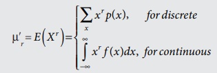
·           Raw moments

·           Central Moments

m_r = E[(X–m_X )^r]

m₁ = E(X) = m_X , the mean of X.

m₁ = E[X–m_X] = 0.

m₂ = E[(X–m_X)²], the variance of X .