Simple Viscoelastic Behavior

Simple Viscoelastic Behavior

All solids are to some extent 'fluid' in that they will flow, even if only a minuscule amount, at working stress levels if enough time passes. Thus stress-strain relationships are actually functions of time (and temperature) and it can be dangerous, even disastrous, to neglect creep effects in such mate-rials as concrete, plastics, wood, or soil when dimensional tolerances must be maintained over time.* Moreover, as we might expect, an increase in temper-ature accelerates viscous flow. All solids turn into liquids or (gases) at their melting point, but long before that, many materials such as metals (which appear elastic at room temperature) will loose stiffness and become viscous** at higher temperatures. Such viscous flow, which can occur under either iso-tropic or deviatoric stress, is easily confused with plastic flow which, as we will see, is a purely deviatoric phenomenon. However, in areas of plastic flow,

(*For example, time-dependent creep distortion of the concrete in Hoover dam (where the load is essentially constant) eventually (after forty years), necessitated replacement of the steel pen-stock liners at great expense. Creep of concrete and wood can reduce effective prestress signifi-cantly (or destroy shallow arches) and the long-term deviatoric creep sometimes thought of as secondary consolidation can, even after hundreds of years, lead to foundation failure as wit-nessed in the Tower of Pisa.

**The melting point of iron, for example, is 1535 ^o C but at only 300 ^o C it begins to flow under load. That is why unprotected steel buildings have a lower fire rating (higher insurance premiums) than concrete or even wooden ones.

)

all distortional resistance is gone* and there is therefore no deviatoric stiffness. An increase in temperature will reduce both the deviatoric stiffness and the yield strength, but it is important to keep the two properties, stiffness and strength, separate in our minds.

Elastic behavior can be modified to include viscous effects by combining dashpots with springs to any degree of complexity deemed necessary to cap-ture the essential stiffness response observed in the laboratory. The simplest such 'models' for viscoelastic behavior combine a single spring and a single dashpot either in series or in parallel. The corresponding 'Maxwell Model' and 'Kelvin Model' are shown in Figures 3.4 and 3.5. In general a separate model may be necessary to depict the observed isotropic and deviatoric behav-ior. This is true, for example, in saturated clays where the volumetric behavior is well represented by a Kelvin model and the deviatoric response by the Maxwell model. The viscoelastic deformation of most solids, however, exhibits much more flow under shear than mean stress. Thus we will discuss the various vis-coelastic models in terms of deviatoric stress and the corresponding distor-tional strain, recognizing that similar models can apply to volumetric behavior

with _m, _m, 3K, and 3 substituted in place of S_ij, e_ij, 2G, and 2.

Since in this book we consider only static loads, the viscoelastic creep (and relaxation) behavior of our models is of primary importance. For many struc-tures, particularly large ones like bridges or the foundations on which they sit, the major part of the stress field in service is due to constant 'dead' loads

anyway. Moreover, even when live loads from wind, temperature changes, earthquakes, or traffic are significant and generate important stress fields, little viscous flow will occur since dashpots cannot react to sudden loads of short duration.* Thus, it is generally a reasonable engineering assumption for viscoelastic solids to calculate live-load stresses from the purely elastic response of the material and the viscous strains from the dead-load part of the stress field neglecting the comparatively transitory effects.**

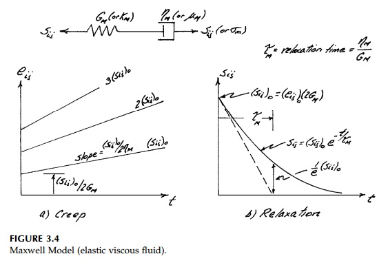
The creep curves for the Maxwell and Kelvin models are shown in Figures 3.4 and 3.5. In each case the derivation of the fundamental stress-strain equation from equilibrium and compatibility is straightforward. For the Maxwell model with the spring and dashpot in series, the stress in each component equals the total applied stress, S_ij, and the total deviatoric strain is the sum of that in each. Therefore, the general equation for the deviatoric Maxwell model is

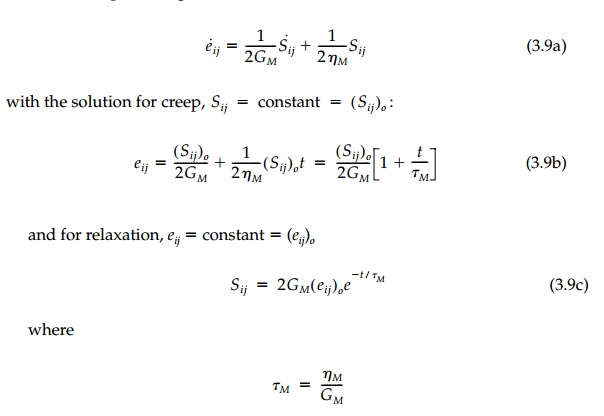
As can be seen in Figure 3.4, the Maxwell model is essentially a fluid. Although it responds elastically and appears to be solid, it flows indefi-nitely under sustained stress. Silly putty is a perfect example of such a material.

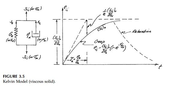
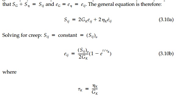
The Kelvin* model where the components are in parallel (Figure 3.5) is, on the other hand, a solid with the dashpot only serving to delay the elastic response. In this case the stress in each component depends on time with the dashpot taking all the stress at t = 0 and the spring only able to accept the stress given up by the dashpot as it strains. Equilibrium and compatibility require

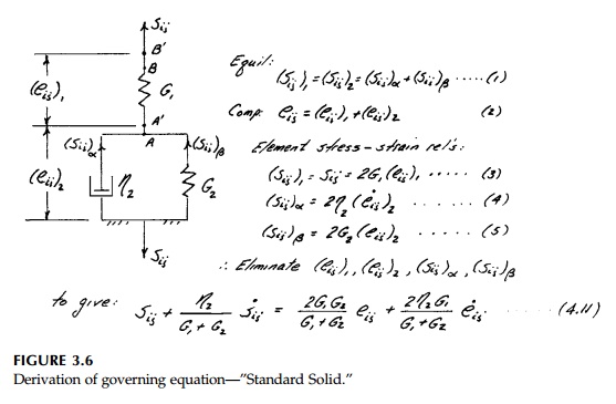
More complicated models can be developed to depict viscoelastic behavior to any degree of sophistication. To illustrate the procedure for determining the basic equations for such hybrid models, the derivation for the 'standard solid' is shown as an example in Figure 3.6 while others are left for home-work problems.

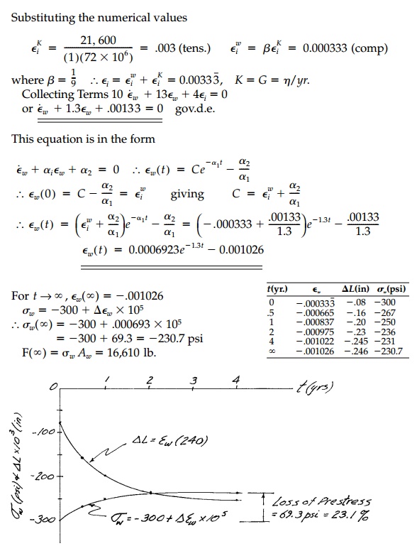
Example 3.2

A six-inch thick wooden bridge deck is post-tensioned with 1 in.² Kevlar tendons with a 1 ft spacing jacked to an initial prestressing force F 21,600 lb as shown. Kevlar can be considered elastic ( E=7.2 x 10⁶ psi), but wood might be an elastic material in isotropic stress and a Kelvin material in deviatoric stress with properties as shown.

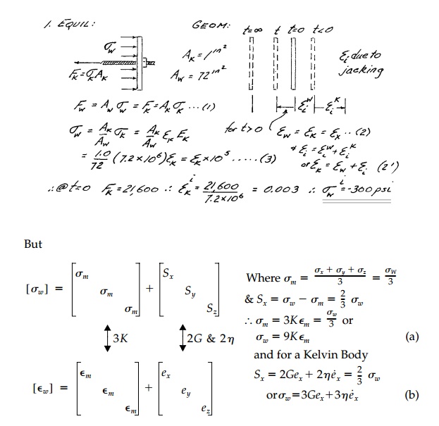
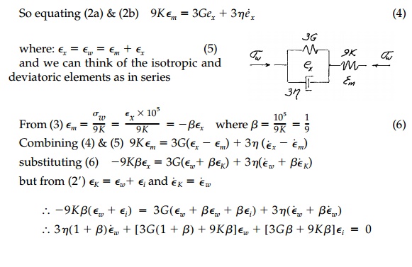
Calculate and plot the stress in the wood and the change in length L as a function of time.

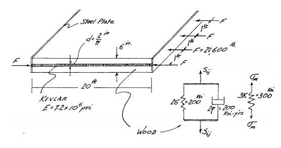
Note:

a)We are concerned only with stress and strain in x direction.

Assume both wood and Kevlar are free to expand in y and z directions.