Fitting Laboratory Data with Viscoelastic Models

Fitting Laboratory Data with Viscoelastic Models

Properties of viscoelastic materials are usually determined in the laboratory with a creep test run at constant temperature. Often a tensile test is used with mea-surements of axial and transverse deformations as a function of time to deter-mine E(t) and v(t). It is better (often necessary) to run separate creep tests in pure states of constant isotropic and deviatoric stress to determine K(t) and G(t) indi-vidually, since for some linear viscoelastic materials, the elastic relationships between E, v, G, and K do not translate directly when they are functions of time.

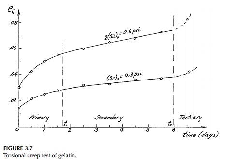
Typical results that were obtained in the laboratory for the creep of gelatin* (in this case a mixture of 10% gelatin, 50% glycerin, and 40% water) in pure shear at room temperature are shown in Figure 3.7. One might decide to fit such curves with a least-squares polynomial, but it is much better, since it is physical and leads to easier mathematics, to combine linear springs and dashpots. As we have seen for the Maxwell, Kelvin, and standard solid models, this leads to a differential equation for the behavior of a particular arrange-ment of springs and dashpots of the form:

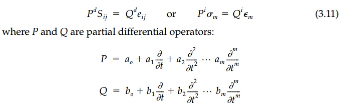
with the coefficients a_i and b_i, various combinations of G_i and _i in the devia-toric case (i.e., for P^d and Q^d), or K_i and _i for the isotropic case (i.e., for Pⁱ and Qⁱ). Thus we can derive time dependent moduli:

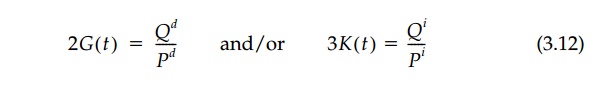
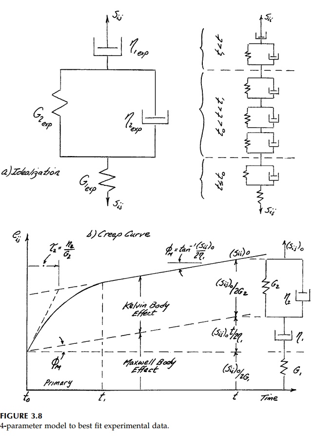
A combination of either n Maxwell models in parallel or n Kelvin models in series with a simple Maxwell model can represent observed linear vis-coelastic behavior to any degree of accuracy desired. However, a 4-parameter model (Burger body) shown in Figure 3.8 will generally capture the funda-mentals of the viscoelastic response with sufficient accuracy for most engi-neering purposes. The deformation at the first time reading, t t_o , is modeled by a spring and primary behavior, t_o < t < t₁, by a single Kelvin body. The contribution of each element is shown in Figure 3.8. Time t₁ is chosen to be where, by eye, the creep curve plotted from the experimental data appears to become a straight line at the angle _M. The initial tangent to the curve at t=t_o is drawn and ₂ determined as shown.

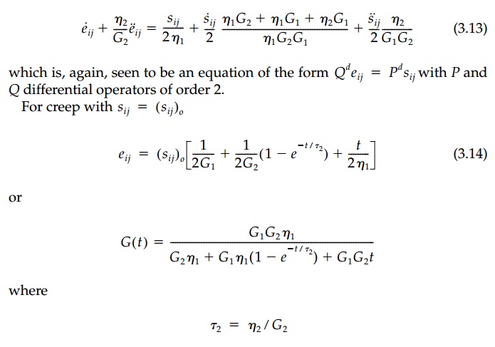
The basic equation for the 4-parameter model is:

From t₁, ₂, and _M as found from the experimental curve drawn by eye to best fit the laboratory data, the element parameters G₁, G₂, , ₂ can be com-puted. If, as in Figure 3.6, the experiment indicates that bonds begin to weaken at large strains, this tertiary behavior can be represented by plastic elements such as those discussed later.