Selected LP Applications: Production Planning and Inventory Control

SELECTED LP APPLICATIONS

This section presents realistic LP models in which the definition of the variables and the construction of the objective function and constraints are not as straight-forward as in the case of the two-variable model. The areas covered by these appli-cations include the following:

1. Urban planning.

2. Currency arbitrage.

3. Investment.

4. Production planning and inventory control.

5. Blending and oil refining.

6. Manpower planning.

Each model is fully developed and its optimum solution is analyzed and interpreted.

4 .Production Planning and Inventory Control

There is a wealth of LP applications to production and inventory control, ranging from simple allocation of machining capacity to meet demand to the more complex case of using inventory to "dampen" the effect of erratic change in demand over a given planning horizon and of using hiring and firing to respond to changes in workforce needs. This section presents three examples. 'The first deals with the scheduling of products using common production facilities to meet demand during a single period, the second deals with the use of inventory in a multiperiod production system to fill future demand, and the third deals with the use of a combined inventory and worker hiring/firing to "smooth" production over a multiperiod planning horizon with fluctuating demand.

Example 2.3-4  (Single-Period Production Model)

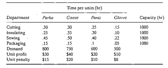
In preparation for the winter season, a clothing company is manufacturing parka and goose overcoats, insulated pants, and gloves. All products are manufactured in four different departments: cutting, insulating, sewing, and packaging. The company has received firm orders for its products. The contract stipulates a penalty for undelivered items. The following table provides the pertinent data of the situation.

Devise an optimal production plan for the company.

Mathematical Model:   The definition of the variables is straightforward. Let

x₁ = number of parka jackets

x₂  = number of goose jackets

x₃  = number of pairs of pants

x₄ = number of pairs of gloves

The company is penalized for not meeting demand. This means that the objective of the problem is to maximize the net receipts, defined as

Net receipts = Total profit - Total penalty

The total profit is readily expressed as 30x₁ + 40x₂ + 20x₃ + 10x₄  The total penalty is a function of the shortage quantities (= demand - units supplied of each product). These quantities can be determined from the following demand limits:

x₁ ≤ 800, x₂≤ 750, x₃≤ 600, x₄ ≤500

A demand is not fulfilled if its constraint is satisfied as a strict inequality. For example, if 650 parka jackets are produced, then x¹ = 650, which leads to a shortage of 800 - 650 = 150 parka jackets. We can express the shortage of any product algebraically by defining a new nonnegative variable-namely,

Sj  = Number of shortage units of product j, j =  1,2,3,4

In this case, the demand constraints can be written as

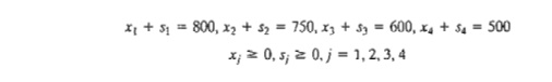
We can now compute the shortage penalty as 15s₁ + 20s₂ + 10s₃ + 8s₄. Thus, the objective func-tion can be written as

To complete the model, the remaining constraints deal with the production capacity restric-tions; namely

.30x₁  + .30x₂ + .25x₃ + .15x₄ ≤  1000            (Cutting)

.25x₁  + .35x₂ + .30x₃ + .lox₄ ≤  1000             (Insulating)

.45x₁  + .50x₂ + aox₃ + .22x₄ ≤  1000             (Sewing)

.15x₁ + .15x₂ + .10x₃ + .05X₄ ≤  1000               (Packaging)

The complete model thus becomes

subject to

.30x₁  + .30x₂ + .25x₃ + .15x₄ ≤ 1000

.25x₁  + .35x₂ + .30x₃ + .10x₄ ≤ 1000

.45x₁ + .50x₂ + .40x₃ + .22x₄ ≤ 1000

.15x₁ + .15x₂ + .10x₃ + .05x₄ ≤ 1000

x₁  + s₁  =  800, x₂ + s₂ = 750, x₃ + s₃ = 600, x₄  + s₄ = 500

xj ≥ 0, sj ≥ 0, j  =  1, 2, 3, 4

Solution:

The optimum solution is z = $64,625, x_l = 850, x₂ = 750, x₃ = 387.5, x₄ = 500, s₁ = s₂ = s₄ = 0, s₃ = 212.5. The solution satisfies all the demand for both types of jackets and the gloves. A shortage of 213 (rounded up from 212.5) pairs of pants will result in a penalty cost of 213 X $10 = $2130.

Example 2.3-5       (Multiple Period Production-Inventory Model)

Acme Manufacturing Company has contracted to deliver horne windows over the next 6 months. The demands for each month are 100,250,190,140,220, and 110 units, respectively. Production cost per window varies from month to month depending on the cost of labor, material, and utilities. Acme estimates the production cost per window over the next 6 months to be $50, $45, $55, $48, $52, and $50, respectively. To take advantage of the fluctuations in manufacturing cost, Acme may elect to produce more than is needed in a given month and hold the excess units for delivery in later months. This, however, will incur storage costs at the rate of $8 per window per month assessed on end-of-month inventory. Develop a linear program to determine the optimum production schedule.

Mathematical Model: The variables of the problem include the monthly production amount and the end-of-month inventory. For i = 1,2, ... , 6, let

x_i= Number of units produced in month i

1i = Inventory units left at the end of month i

The relationship between these variables and the monthly demand over the six-month horizon is represented by the schematic diagram in Figure 2.5. The system starts empty, which means that

1₀  = 0.

The objective function seeks to minimize the sum of the production and end-of-month in-ventory costs. Here we have,

Total production cost = 50x₁  + 45x₂ + 55x₃  + 48x₄ + 52x_s + 50x₆

Total inventory cost = 8(I₁ + l₂ + I₃ + 1₄ + 1₅  + I₆ )

Thus the objective function is

Minimize z = 50x₁  + 45x₂ + 55x₃ + 48x₄ + 52x_s + 50x₆+ 8( I₁  + 1₂  + I₃ + 1₄  + Is + I₆ )

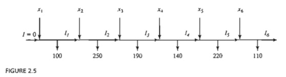
Schematic representation of the production-inventory system

The constraints of the problem can be determined directly from the representation in Figure 2.5. For each period we have the following balance equation:

Beginning inventory + Production amount -        Ending inventory = Demand

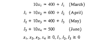
This is translated mathematically for the individual months as

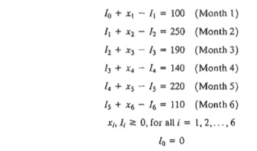
For the problem, 1₀ = 0 because the situation starts with no initial inventory. Also, in any optimal solution, the ending inventory h will be zero, because it is not logical to end the horizon with positive inventory, which can only incur additional inventory cost without serving any purpose.

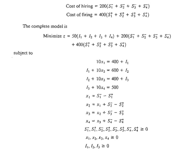
The complete model is now given as

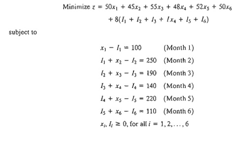
Optimum solution of the production.inventory problem

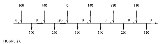
Solution:

The optimum solution is summarized in Figure 2.6. It shows that each month's demand is satis-fied directly from the month's production, except for month 2 whose production quantity of 440 units covers the demand for both months 2 and 3. The total associated cost is z = $49,980.

Example 2.3-6        (Multiperiod Production Smoothing Model)

A company will manufacture a product for the next four months: March, April, May, and June. The demands for each month are 520, 720, 520, and 620 units, respectively. The company has a steady workforce of 10 employees but can meet fluctuating production needs by hiring and fir-ing temporary workers, if necessary. The extra costs of hiring and firing in any month are $200 and $400 per worker, respectively. A permanent worker can produce 12 units per month, and a temporary worker, lacking comparable experience, only produce 10 units per month. TIle com-pany can produce more than needed in any month and carry the surplus over to a succeeding month at a holding cost of $50 per unit per month. Develop an optimal hiring/firing policy for the company over the four-month planning horizon.

Mathematical Model: This model is similar to that of Example 2.3-5 in the general sense that each month has its production, demand, and ending inventory. There are two exceptions: (1) ac-counting for the permanent versus the temporary workforce, and (2) accounting for the cost of hiring and firing in each month.

Because the permanent 10 workers cannot be fired, their impact can be accounted for by subtracting the units they produce from the respective monthly demand. The remaining demand, if any, is satisfied through hiring and firing of temps. From the standpoint of the model, the net demand for each month is

Demand for March  = 520 - 12 X  10 = 400 units

Demand for April  = 720 - 12 X  10 = 600 units

Demand for May  = 520 - 12 X  10 = 400 units

Demand for June = 620 - 12 X  10 = 500 units

For i = 1,2,3,4, the variables of the model can be defined as

x_i = Net number of temps at the start of month i after any hiring or firing

S_i =  Number of temps hired or fired at the start of month i

Ii =    Units of ending inventory for month i

The variables x_i and Ii, by definition, must assume nonnegative values. On the other hand, the variable S_i can be positive when new temps are hired, negative when workers are fired, and zero if no hiring or firing occurs. As a result, the variable must be unrestricted in sign, This is the first instance in this chapter of using an unrestricted variable. As we will see shortly, special substitu-tion is needed to allow the implementation of hiring and firing in the model.

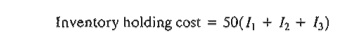
The objective is to minimize the sum of the cost of hiring and firing plus the cost of holding inventory from one month to the next. The treatment of the inventory cost is similar to the one given in Example 2.3-5-namely,

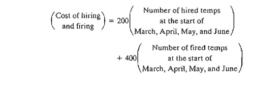
(Note that I4 = 0 in the optimum solution.) The cost of hiring and firing is a bit more involved. We know that in any optimum solution, at least 40 temps (= 400/10) must be hired at the start of March to meet the month's demand. However, rather than treating this situation as a special case, we can let the optimization process take care of it automatically. Thus, given that the costs of hiring and firing a temp are $200 and $400, respectively, we have

To translate this equation mathematically, we will need to develop the constraints first.

The constraints of the model deal with inventory and hiring and firing. First we develop the inventory constraints. Defining x_i as the number of temps available in month i and given that the productivity of a temp is 10 units per month, the number of units produced in the same month is lOXi' Thus the inventory constraints are

Next, we develop the constraints dealing with hiring and firing. First, note that the temp work-force starts with x₁ workers at the beginning of March. At the start of April, x₁ will be adjusted (up or down) by S₂ to generate x₂. The same idea applies to x₃ and x₄. These observations lead to the following equations

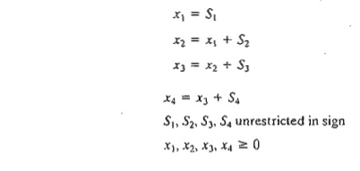
The variables S1, S₂, S3, and S4 represent hiring when they are strictly positive and firing when they are strictly negative. However, this "qualitative" information cannot be used in a mathematical expression. Instead, we use the following substitution:

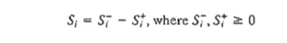
The unrestricted variable Si is now the difference between two nonnegative variables S_i^- and S_i⁺. We can think of S_i^-  as the number of temps hired and S_i⁺  as the number of temps fired. For example, if S_i^-  = 5 and S_i⁺  = 0 then S_i = 5 - 0 = +5, which represents hiring. If S_i^-  = 0 and S_i⁺  = 7 then S_i = 0 - 7 = -7, which represents firing. In the first case, the corresponding cost of hiring is 200 S_i⁺  = 200 X 5 = $1000 and in the second case the corresponding cost of firing is 400 S_i⁺  = 400 X 7 = $2800. This idea is the basis for the development of the objective function.

First we need to address an important point: What if both S_i^-  and S_i⁺  are positive? The answer is that this cannot happen because it implies that the solution calls for both hiring and firing in the same month. Interestingly, the theory of linear programming (see Chapter 7) tells us that S_i^-  and S_i⁺  can never be positive simultaneously, a result that confirms intuition.

We can now write the cost of hiring and firing as follows:

Solution:

The optimum solution is z = $19,500, x₁ = 50, x₂ = 50, x₃ = 45, x₄ = 45, 5, S_i^-  = 50, S_i⁺  = 5, I₁ = 100, I₃ = 50. All the remaining variables are zero. The solution calls for hiring 50 temps in March (S_i^-  = 50) and holding the workforce steady till May, when 5 temps are fired (S_i⁺  = 5). No further hiring or firing is recommended until the end of June, when, presumably, all temps are terminated. This solution requires 100 units of inventory to be carried into May and 50 units to be carried into June.

PROBLEM SET 2.30

Tooleo has contracted with AutoMate to supply their automotive discount stores with wrenches and chisels. AutoMate's weekly demand consists of at least 1500 wrenches and 1200 chisels. Tooleo cannot produce all the requested units with its present one-shift capacity and must use overtime and possibly subcontract with other tool shops. The result is an increase in the production cost per unit, as shown in the following table. Market de-mand restricts the ratio of chisels to wrenches to at least 2:1.

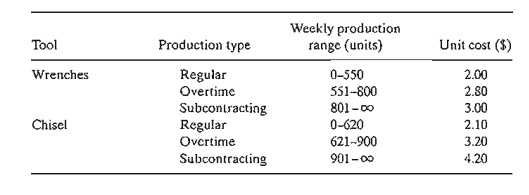
                                a. Formulate the problem as a linear program, and determine the optimum production schedule for each tool.

                                b. Relate the fact that the production cost function has increasing unit costs to the va-lidi ty of the modeL

2. Four products are processed sequentially on three machines. The following table gives the pertinent data of the problem.

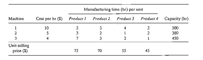
Formulate the problem as an LP model, and find the optimum solution.

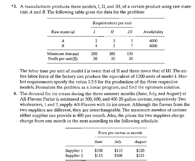
The production rates in units per hour are 1.25 and 1 for products A and B, respec-tively. All demand must be met. However, demand for a later month may be filled from the production in an earlier one. For any carryover from one month to the next, holding costs of $.90 and $.75 per unit per month are charged for products A and B, respectively. The unit production costs for the two products are $30 and $28 for A and B, respectively. Determine the optimum production schedule for the two products.

*7. The manufacturing process of a product consists of two successive operations, I and II. The following table provides the pertinent data over the months of June, July, and August:

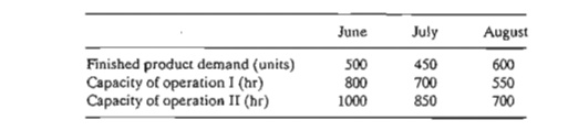
Producing a unit of the product takes .6 hour on operation I plus .8 hour on operation II. Overproduction of either the semifinished product (operation I) or the finished product (operation II) in any month is allowed for use in a later month. The corre-sponding holding costs are $.20 and $.40 per unit per month. The production cost varies by operation and by month. For operation 1, the unit production cost is $10, $12, and $11 for June, July, and August. For operation 2, the corresponding unit production cost is $15, $18, and $16. Determine the optimal production schedule for the two operations over the 3-month horizon.

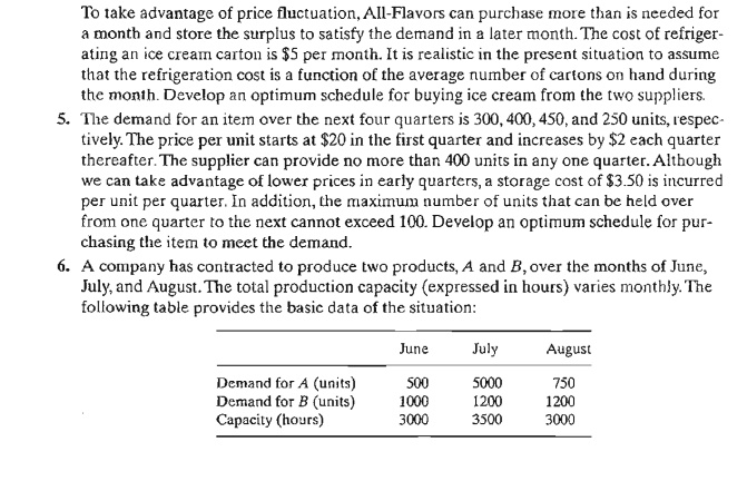
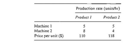
8. Two products are manufactured sequentially on two machines. The time available on each machine is 8 hours per day and may be increased by up to 4 hours of overtime, if necessary, at an additional cost of $100 per hour. The table below gives the production rate on the two machines as well as the price per unit of the two products. Determine the optimum production schedule and the recommended use of overtime, if any.