Chapter: Operations Research: An Introduction : Modeling with Linear Programming
Computer Solution With Solver and AMPL
COMPUTER SOLUTION WITH SOLVER AND AMPL
In practice, where typical linear programming models may involve thousands of variables and constraints, the only feasible way to solve such models is to use the computer. This section presents two distinct types of popular software: Excel Solver and AMPL. Solver is particularly appealing to spreadsheet users. AMPL is an algebraic modeling language that, like any other programming language, requires more exper-tise. Nevertheless, AMPL, and other similar languages, offer great flexibility in model-ing and executing large and complex LP models. Although the presentation in this section concentrates on LPs, both AMPL and Solver can be used with integer and non-linear programs, as will be shown later in the book.
1. LP Solution with Excel Solver
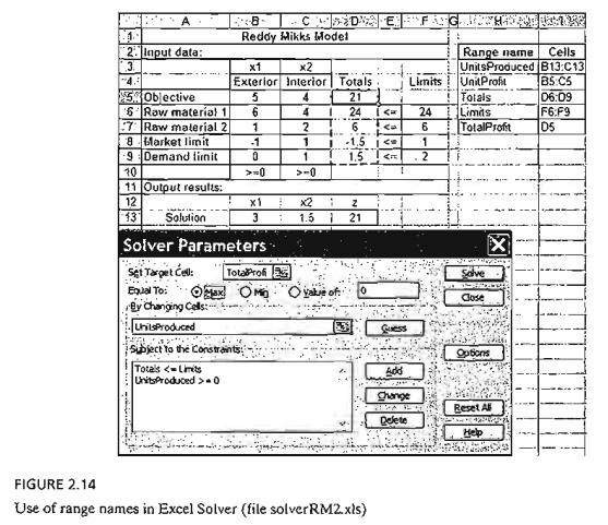
In Excel Solver, the spreadsheet is the input and output medium for the LP. Figure 2.12
shows the layout of the data for the Reddy Mikks model (file solverRM1.xls). The top of the figure includes four types of information: (1) input data cells (shaded areas,

B5:C9 and F6:F9), (2) cells representing the variables and the objective function we seek to evaluate (solid rectangle cells, B13:013), (3) algebraic definitions of the objec-tive function and the left-hand side of the constraints (dashed rectangle cells, 05:09), and (4) cells that provides explanatory names or symbols. Solver requires the first three types only. The fourth type enhances the readability of the model and serves no other purpose. The relative positioning of the four types of information on the spread-sheet need not follow the layout shown in Figure 2.12. For example, the cells defining the objective function and the variables need not be contiguous, nor do they have to be placed below the problem. What is important is that we know where they are so they can be referenced by Solver. Nonetheless, it is a good idea to use a format similar to the one suggested in Figure 2.12, because it makes the model more readable.
How does Solver link to the spreadsheet data? First we provide equivalent "alge-braic" definitions of the objective function and the left-hand side of the constraints using the input data (shaded cells B5:C9 and F6:F9) and the objective function and variables (solid rectangle cells B13:013), and then we place the resulting formulas in the appropriate cells of the dashed rectangle D5:09. The following table shows the original LP functions and their placement in the appropriate cells:
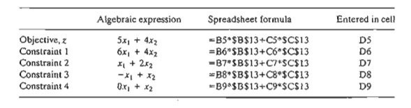
Actually, you only need to enter the formula for cell 05 and then copy it into cells D6:09. To do so correctly, the fixed references $B$13 and $C$13 representing xl and x2 must be used. For larger linear programs, it is more efficient to enter
=SUMPROOUCf(B5:C5,$B$13:$C$13)
in cell D5 and copy it into cells D6:D9.
All the elements of the LP model are now ready to be linked with Solver. From Excel's Tools menu, select Solver4 to open the Solver Parameters dialogue box shown in the middle of Figure 2.12. First, you define the objective function, z, and the sense of optimization by entering the following data:
Set Target Cell: $D$5
Equal To: ʘ Max
By Changing Cells: $B$13:$C$13
This information tells Solver that the variables defined by cells $B$13 and $C$13 are determined by maximizing the objective function in cell $D$5.
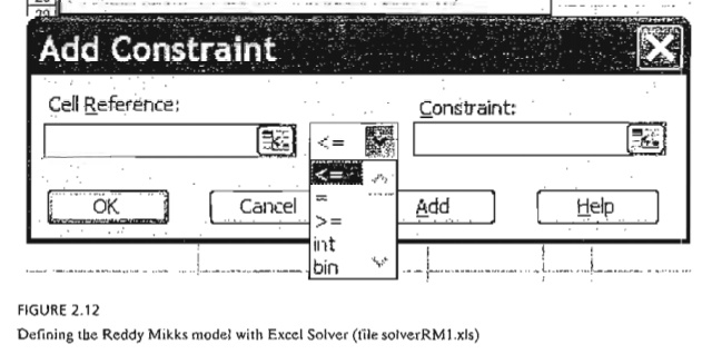
The next step is to set up the constraints of the problems by clicking Add in the Solver Parameters dialogue box. The Add Constraint dialogue box will be displayed (see the bottom of Figure 2.12) to facilitate entering the elements of the constraints (left-hand side, inequality type, and right-hand side) as
$D$6:$D$9<=$F$6:$F$9
A convenient substitute to typing in the cell ranges is to highlight cells D6:D9 to enter the left-hand sides and then cells F6:F9 to enter the right-hand sides. The same proce-dure can be used with Target Cell.
The only remaining constraints are the nonnegativity restrictions, which are added to the model by clicking Add in the Add Constraint dialogue box to enter
$B$13:$C$13>=0
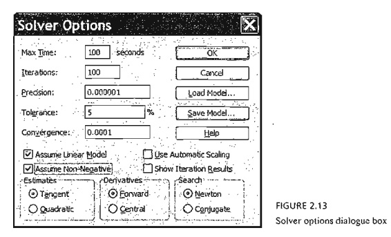
Another way to enter the nonnegative constraints is to click Options on the Solver Pa-rameters dialogue box to access the Solver Options dialogue box (see Figure 2.13) and then check ![]() Assume Non-Negative. While you are in the Solver Options box, you also need to check
Assume Non-Negative. While you are in the Solver Options box, you also need to check ![]() Assume Linear Model.
Assume Linear Model.
In general, the remaining default settings in Solver Options need not be changed. However, the default precision of .000001 may be set too "high" for some problems, and Solver may return the message "Solver could not find a feasible solution" when in fact the problem does have a feasible solution. In such cases, the precision needs to be adjusted to reflect less precision. If the same message persists, then the problem may be infeasible.
For readability, you can use descriptive Excel range names instead of cell names. A range is created by highlighting the desired cells, typing the range name in the top left box of the sheet, and then pressing Return. Figure 2.14 (file solverRM2.xls) provides the details with a summary of the range names used in the model. You should contrast file solverRM2.xls with file solverRM1.xls to see how ranges are used in the formulas.
To solve the problem, click Solve on Solver Parameters (figure 2.14). A new di-alogue box, Solver Results, will then give the status of the solution. If the model setup is correct, the optimum value of z will appear in cell D5 and the values of Xl and X2 will go to cells B13 and C13, respectively. For convenience, we use cell Dl3 to exhibit the optimum value of z by entering the formula =D5 in cell DB to display the entire opti-mum solution in contiguous cells.
If a problem has no feasible solution, Solver will issue the explicit message "Solver could not find a feasible solution." If the optimal objective value is unbounded, Solver will issue the somewhat ambiguous message "The Set Cell values do not con-verge." In either case, the message indicates that there is something wrong with the for-mulation of the model, as will be discussed in Section 3.5.
The Solver Results dialogue box will give you the opportunity to request further details about the solution, including the important sensitivity analysis report. We will discuss these additional results in Section 3.6.4.
The solution of the Reddy Mikks by Solver is straightforward. Other models may 2.4. require a "bit of ingenuity" before they can be defined in a convenient manner. A class
of LP models that falls in this category deals with network optimization, as will be demonstrated in Chapter 6.
PROBLEM SET 2.4A
1. Modify the Reddy Mikks Solver model of Figure 2.12 to account for a third type of paint named “marine.” Requirements per ton of raw materials 1 and 2 are .5 and .75 ton, re-spectively. The daily demand for the new paint lies between .5 ton and 1.5 tons. The profit per ton is $3.5 (thousand).
2. Develop the Excel Solver model for the following problems:
b.Problem 16, Set 2.2a
c.The urban renewal model of Example 2.3-1.
*d. The currency arbitrage model of Example 2.3-2. (Hint: You will find it convenient to use the entire currency conversion matrix rather than the top diagonal elements only. Of course, you generate the bottom diagonal elements by using appropriate Excel formulas.)
e.The multi-period production-inventory model of Example 2.3-5.
2. LP Solution with AMPl
This section provides a brief introduction to AMPL. The material in Appendix A pro-vides detailed coverage of AMPL syntax and will be cross-referenced opportunely with the presentation in this section as well as with other AMPL presentations throughout the book.
Four examples are presented here: The first two deal with the basics of AMPL, and the remaining two demonstrate more advanced usages to make a case for the ad-vantages of AMPL.
Reddy Mikks Problem-a Rudimentary Model. AMPL provides a facility for modeling an LP in a rudimentary long-hand format. Figure 2.15 gives the self-explanatory code
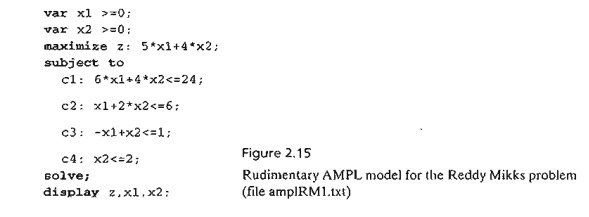
for the Reddy Mikks model (file ampIRM1.txt). All reserved keywords are in bold. All other names are user generated. The objective function and each of the constraints must be given a distinct user-generated name followed by a colon. Each statement closes with a semi-colon.
This rudimentary AMPL model is too specific in the sense that it requires devel-oping a new code each time the data of the problem are changed. For practical prob-lems with hundreds (even thousands) of variables and constraints, this long-hand format is cumbersome. AMPL alleviates this difficulty by dividing the problem into two components: (1) A general model that expresses the problem algebraically for any desired number of variables and constraints, and (2) specific data that drive the algebraic model. We will use the Reddy Mikks model to demonstrate the basic ideas ofAMPL.
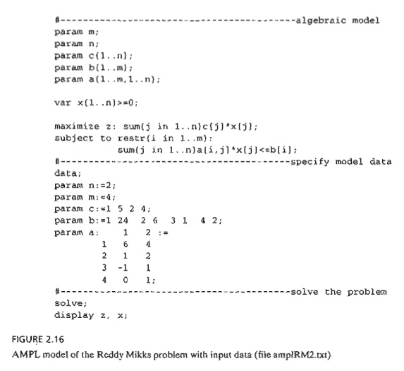
Reddy Mikks Problem-an Algebraic Model. Figure 2.16 lists the statements of the model (file ampIRM2.txt). The file must be strictly text (ASCII). Comments are preceded with # and may appear anywhere in the model. The language is case sensitive and all its keywords (with few exceptions) must be in lower case. (Section A.2 provides more details.)
The algebraic model in AMPL views the general Reddy Mikks problem in the following generic format
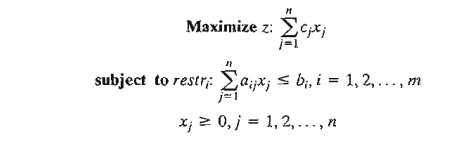
It assumes that the problem has n variables and m constraints. It gives the objective function and constraint i the (arbitrary) names z and restri. The rest of the parameters cj, bi, and aij are self-explanatory.
The model starts with the param statements that declare m, n.,c, b, and aij as parameters (or constants) whose specific values are given in the input data sec-tion of the modeL It translates cj(j = 1,2, , n) as c {1. . n}, bi (i = 1,2, ... , m) as b{1. .m}, and aij(i = 1,2, ... ,m , j = 1,2, ,n) as a{1 .. m,1. .n}. Next, the variables xj (j = 1,2, ... , n) together with the nonnegativity restriction are defined by the var statement

If >=0 is removed from the definition of xj, then the variable is assumed unrestricted. The notation in {} represents the set of subscripts over which a param or a var is defined.
After defining all the parameters and the variables, we can develop the model it-self. The objective function and constraints must each carry a distinct user-defined name followed by a colon (:). In the Reddy Mikks model the objective is given the name z: preceded by maximi ze, as the following AMPL statement states:

Note the use of the brackets [] for representing the subscripts.
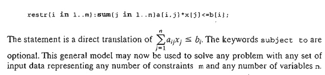
Constraint i is given the root name restr indexed over the set {1 .. m}:
The data; section allows tailoring the model to the specific Reddy Mikks prob-lem. Thus, param n: =2; and param m: =4; tell AMPL that the problem has 2 variables and 4 constraints. Note that the compound operator : = must be used and that the statement must start with the keyword paramo For the single-subscripted parameter c, each element is represented by the subscript j followed by cj separated by a blank space.Thuss, the two values C1 = 5 and C2 = 4 translate to
param c:= 1 5 2 4;
The data for parameter b are entered in a similar manner.
For the double-subscripted parameter a, the top line defines the subscript j, and the subscript i is entered at the start of each row as
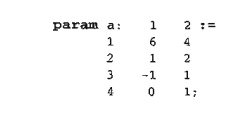
In effect, the data aij read as a two-dimensional matrix with its rows designating i and its columns designatingj. Note that a semicolon is needed only at the end of all aij data.
The model and its data are now ready. The command solve; invokes the solu-tion and the command display z, x; provides the solution.
To execute the model, first invoke AMPL (by clicking ampI.exe in the AMPL di-rectory). At the ampl prompt, enter the following model command, then press Return:
ampl: model AmplRM2. txt;
The output of the system will then appear on the screen as follows:
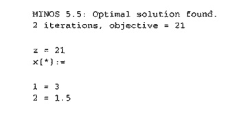
The bottom four lines are the result of executing display z, x; .
Actually, AMPL allows separating the algebraic model and the data into two inde-pendent files. This arrangement is advisable because once the model has been developed, only the data file needs to be changed. (See the end of Section A.2 for details.) In this book, we elect not to separate the model and data files, mainly for reasons of compactness.
The Arbitrage Problem. The simple Reddy Mikks model introduces some of the basic elements of AMPL. The more complex arbitrage model of Example 2.3-2 offers the opportunity to introduce additional AMPL capabilities that include: (1) imposing conditions on the elements of a set, (2) use of if then else to represent conditional values, (3) use of computed parameters, and (4) use of a simple print statement to retrieve output. These points are also discussed in more detail in Appendix A.
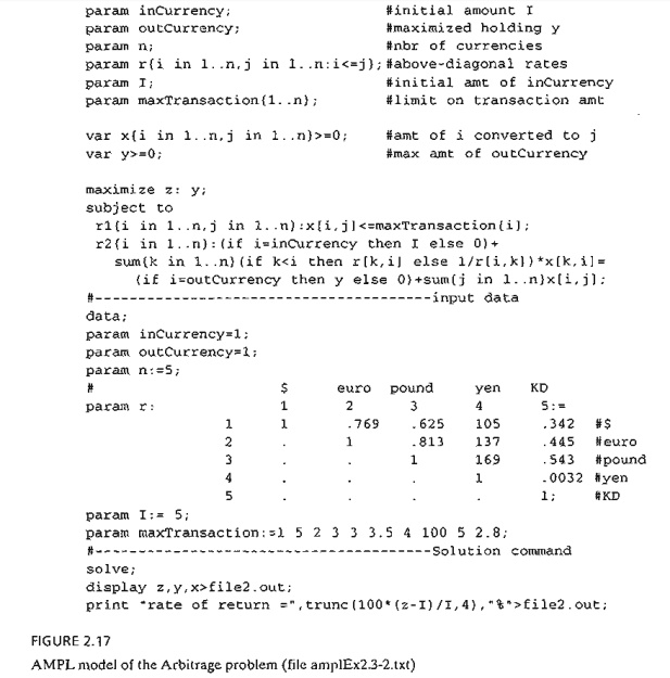
FIGURE 2.17
AMPL model of the Arbitrage problem (file ampIEx2.3-2.txt)
Figure 2.17 (file ampIEx2.3-2.txt) gives the AMPL code for the arbitrage prob-lem. The model is general in the sense that it can be used to maximize the final holdings y of any currency, named outCurrency, starting with an initial amount I of another currency, named inCurrency. Additionally, any number of currencies, n, can be in-volved in the arbitrage process.
The exchange rates are defined as
param r{i in 1. .n,j in 1. .n:i<=j];
The definition gives only the diagonal and above-diagonal elements by imposing the condition i<=j (preceded by a colon) on the set (i in 1 .. n, j in 1 .. n). With this definition, reciprocals are used to compute the below-diagonal rates, as will be shown shortly.
The variable xij, representing the amount of currency i converted to currency j, is defined as
var x{i in 1 ..n,j in 1 .. n>=0;
The model has two sets of constraints: The first set with the root name rl sets the limits on the amounts of any currency conversion transaction by using the statement
r1{i in 1 .. n,j in 1 .. n}: x[i,j]<=maxTransaction[i];
The second set of constraints with the root name r2 is a translation of the restriction
(Input to currency i) = (Output from currency j)
Its statement is given as
r2{i in 1 .. n} :
(if i=inCurrency then I else 0)+
sum{k in l ..n}{if k<i then r[k,i] else l/r[i,k])*x[k,i]
=(if i=outCurrency then y else o)+surn{j in 1 .. n}x[i,j];
This type of constraints is ideal for the use of the special construct if then else to specify conditional values. In the left-hand side of the constraint, the expression
(if i=inCurrency then 1 else 0)
says that in the constraint for the input currency (i=inCurrency) there is an external input I, else the external input is zero. Next, the expression
sum{k in l .. n} (if k<i then r[k,i] else 1/r[i,kJ)*x[k,i]
The if-expression in the right-hand side of constraint r2 can be explained in a similar manner - namely,
(if i=outCurrency then y else 0)
says that the external output is y for outCurrency and zero for all others.
We can enhance the readability of constraints r2 by defining the following computed parameter (see Section A.3) that defines the entire exchange rate table:
Pararn rate(k in 1 .. n,i in 1 .. n}
=(if k<i then r[k,iJ else l/r[i,k])
In this case, constraints r2 become
In the data; section, inCurrency and outCurrency each equal 1, which means that the problem is seeking the maximum dollar output using an initial amount of $5 million. In general, inCurrency and outC\lrrency may designate any distinct curren-cies. For example, setting inCurrency equal to 2 and outCurrency equal to 4 maxi-mizes the yen output given a 5 million euros initial investment.
The unspecified entries of param r are flagged in AMPL with dots (.). These values are then overridden either by using the reciprocal as shown in Figure 2.17 or through the use of the computed parameter ra te as shown above. The alternative to using dots is to unnecessarily compute and enter the below-diagonal elements as data.
The display statement sends the output to file file2.out instead of defaulting it to the screen. The print statement computes and truncates the rate of return and sends the output to file file2.out. The print statement can also be formatted using printf, just as in any higher level programming language. (See Section A.S.2 for details.)
It is important to notice that input data in AMPL need not be hard-coded in the model, as they can be retrieved from external files, spreadsheets, and databases (see Section A.S for details). This is crucial in the arbitrage model, where the volaThe ex-change rates must often be accepted within less than 10 seconds. By allowing the AMPL model to receive its data from a database that automatically updates the ex-change rates, the model can provide timely optimal solutions.
The Bus Scheduling Problem. The bus scheduling problem of Example 2.3-8 provides an interesting modeling situation in AMPL. Of course, we can always use a two-subscripted parameter, similar to parameter a in the Reddy Mikks model in Section 2.4.2 (Figure 2.16), but this may be cumbersome in this case. Instead, we can take advantage of the special structure of the constraints and use conditional expressions to represent them implicitly.
AMPL offers a wide range of programming capabilities. For example, the input/output data can be secured from/sent to external files, spreadsheets, and data-bases and the model can be executed interactively for a wide variety of options that allow testing different scenarios. The details are given in Appendix A. Also, many AMPL models are presented throughout the book with cross references to the materi-al in Appendix A to assist you in understanding these options.
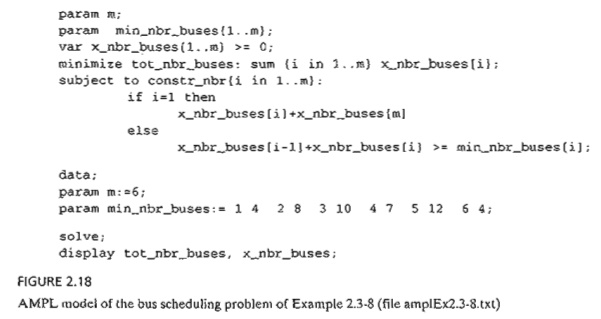
AMPL model of the bus scheduling problem of Example 2.3-8 (file ampIEx2.3-8.txt)
PROBLEM SET 2.4B
Related Topics