Selected LP Applications: Additional Applications

SELECTED LP APPLICATIONS

This section presents realistic LP models in which the definition of the variables and the construction of the objective function and constraints are not as straight-forward as in the case of the two-variable model. The areas covered by these appli-cations include the following:

1. Urban planning.

2. Currency arbitrage.

3. Investment.

4. Production planning and inventory control.

5. Blending and oil refining.

6. Manpower planning.

Each model is fully developed and its optimum solution is analyzed and interpreted.

6. Additional Applications

The preceding sections have demonstrated the application of LP to six representative areas. The fact is that LP enjoys diverse applications in an enormous number of areas. The problems at the end of this section demonstrate some of these areas, ranging from agriculture to military applications. This section also presents an interesting application that deals with cutting standard stocks of paper rolls to sizes specified by customers.

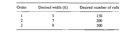
Example 2.3-9   (Trim Loss or Stock Slitting)

The Pacific Paper Company produces paper rolls with a standard width of 20 feet each. Special customer orders with different widths are produced by slitting the standard rolls. Typical orders (which may vary daily) are summarized in the following table:

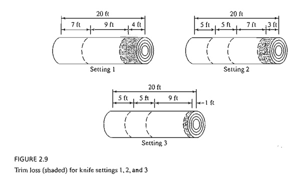
In practice, an order is filled by setting the knives to the desired widths. Usually, there are a number of ways in which a standard roll may be slit to fill a given order. Figure 2.9 shows three feasible knife settings for the 20-foot roll. Although there are other feasible settings, we limit the discussion fOT the moment to settings 1,2, and 3 in Figure 2.9. We can combine the given settings in a number of ways to fill orders for widths 5,7, and 9 feet. The following are examples of feasible combinations:

                    1. Slit 300 (standard) rolls using setting 1 and 75 rolls using setting 2.

                    2. Slit 200 rolls using setting 1 and 100 rolls using setting 3.

Which combination is better? We can answer this question by considering the "waste" each combination generates. In Figure 2.9 the shaded portion represents surplus rolls not wide enough to fill the required orders. These surplus rolls are referred to as trim loss. We can evalu-ate the "goodness" of each combination by computing its trim loss. However, because the surplus rolls may have different widths, we should base the evaluation on the trim loss area rather than on the number of surplus rolls. Assuming that the standard roll is of length L feet, we can com-pute the trim-loss area as follows:

Combination 1: 300 (4 X L)  + 75 (3  X L)  = 1425L ft²

Combination 2: 200 (4  X  L)  + 100 (1  X  L)  = 900L ft ²

These areas account only for the shaded portions in Figure 2.9. Any surplus production of the 5-, 7- and 9-foot rolls must be considered also in the computation of the trim-loss area. In

combination 1, setting 1 produces a surplus of 300 - 200 = 100 extra 7-foot rolls and setting 2 produces 75 extra 7-foot rolls. Thus the additional waste area is 175 (7 x L) = 1225L ft². Combination 2 does not produce surplus rolls of the 7- and 9-foot rolls but setting 3 does produce 200 - 150 = 50 extra 5-foot rolls, with an added waste area of 50 (5 x L) = 250L ft²• As a re-sult we have

Total trim-loss area for combination 1 = 1425L + 1225L = 2650L ft²

Total trim-loss area for combination 2 = 900L + 250L = 1150L ft²

Combination 2 is better, because it yields a smaller trim-loss area.

Mathematical Model: The problem can be summarized verbally as determining the knife-set-ting combinations (variables) that will fill the required orders (constraints) with the least trim-loss area (objective).

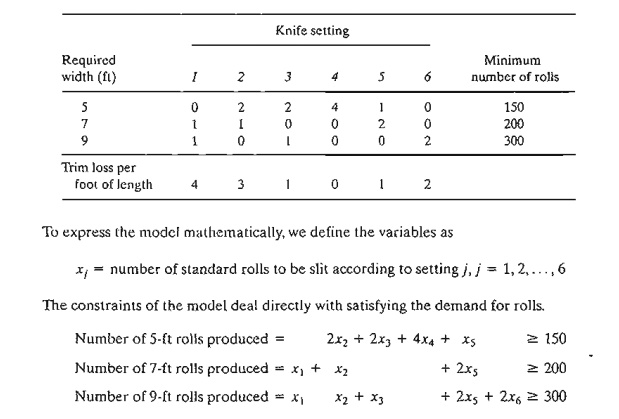
The definition of the variables as given must be translated in a way that the mill operator can use. Specifically, the variables are defined as the number of standard rolls to be slit according to a given knife setting. This definition requires identifying all possible knife settings as summarized in the following table (settings 1,2, and 3 are given in Figure 2.9). You should convince yourself that settings 4,5, and 6 are valid and that no "promising" settings have been excluded. Remember that a promising setting cannot yield a trim-loss roll of width 5 feet or larger.

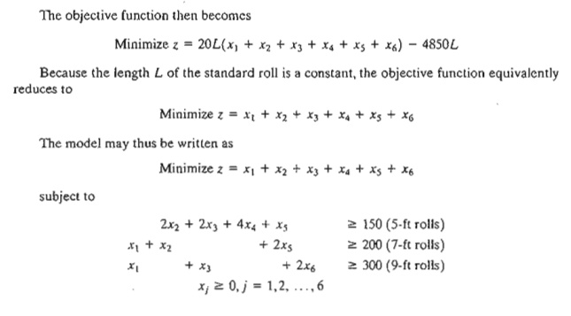
To construct the objective function, we observe that the total "trim loss area is the difference between the total area of the standard rolls used and the total area representing all the orders. Thus

Total area of standard rolls = 20L(x₁  + x₂  + x₃  + x₄  + x₅  + x₆)

Total area of orders = L(150 x 5 + 200 x 7 + 300 x 9)  = 4850L

Solution:

The optimum solution calls for cutting 12.5 standard rolls according to setting 4, 100 according to setting 5, and 150 according to setting 6. The solution is not impIementable because x₄ is nonin-teger. We can either use an integer algorithm to solve the problem (see Chapter 9) or round X4 conservatively to 13 rolls.

Remarks. The trim-loss model as presented here assumes that all the feasible knife settings can be determined in advance. This task may be difficult for large problems, and viable feasible com-binations may be missed. The problem can be remedied by using an LP model with imbedded in-teger programs designed to generate promising knife settings on demand until the optimum solution is found. This algorithm, sometimes referred to as column generation, is detailed in Comprehensive Problem 7-3, Appendix E on the CD. The method is rooted in the use of (rea-sonably advanced) linear programming theory, and may serve to refule the argument that, in practice, it is unnecessary to learn LP theory.

PROBLEM SET 2.3G

*1. Consider the trim-loss model of Example 2.3-9.

a)     If we slit 200 rolls using setting 1 and 100 rolls using setting 3, compute the associat-ed trim-loss area.

b)    Suppose that the only available standard roll is 15 feet wide. Generate all possible knife settings for producing 5-, 7-, and 9-foot rolls, and compute the associated trim loss per foot length.

c)     In the original model, if the demand for 7-foot rolls is decreased by 80, what is the minimum number of standard 20-foot rolls that will be needed to fill the demand for of all three types of rolls?

d)    In the original model, if the demand for 9-foot rolls is changed to 400, how many ad-ditional standard 20-foot rolls will be needed to satisfy the new demand?

2. Shelf Space Allocation. A grocery store must decide on the shelf space to be allocated to each of five types of breakfast cereals.lhe maximum daily demand is 100,85,140,80, and 90 boxes, respectively. The shelf space in square inches for the respective boxes is 16,24, 18,22, and 20. The total available shelf space is 5000 in². The profit per unit is $1.10, $1.30, $1.08, $1.25, and $1.20, respectively. Determine the optimal space allocation for the five cereals.

3. Voting on Issues. In a particular county in the State of Arkansas, four election issues are on the ballot: Build new highways, increase gun control, increase farm subsidies, and increase gasoline tax. The county includes 100,000 urban voters, 250,000 suburban voters, and 50,000 rural volers, all with varying degrees of support for and opposition to election issues. For example, rural voters are opposed to gun control and gas tax and in favor of road building and fann subsidies. The county is planning a TV advertising campaign with a budget of $100,000 at the cost of $1500 per ad. The following table summarizes the impact of a single ad in terms of the number of pro and can votes as a function of the different issues:

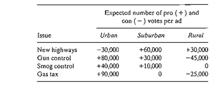
An issue will be adopted if it garners at least 51 % of the votes. Which issues will be ap-proved by voters, and how many ads should be allocated to these issues?

4. Assembly-Line Balancing. A product is assembled from three different parts. The parts are manufactured by two departments at different production rates as given in the following table:

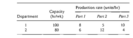
Determine the maximum number of final assembly units that can be produced weekly. (Hint. Assembly units = min {units of part 1, units of part 2, units of part 3}. Maximize z = min{x₁, x2} is equivalent to max z subject to z ≤ x₁ and z ≤ x₂')

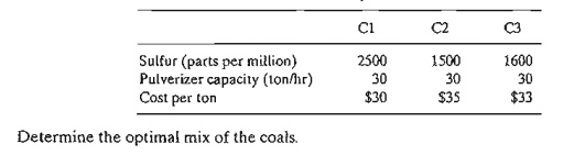
5. Pollution Control. Three types of coal, C1, C2, and C3, are pulverized and mixed together to produce 50 tons per hour needed to power a plant for generating electricity. The burning of coal emits sulfur oxide (in parts per million) which must meet the Environmental Protection Agency (EPA) specifications of at most 2000 parts per million. The following table summarizes the data of the situation:

*6. Traffic Light Control. (Stark and Nicholes, 1972) Automobile traffic from three high-ways, HI, H2, and H3, must stop and wait for a green light before exiting to a toll road. The tolls are $3, $4, and $5 for cars exiting from HI, H2, and H3, respectively. The flow rates from HI, H2, and H3 are 500,600, and 400 cars per hour. The traffic light cycle may not exceed 2.2 minutes, and the green light on any highway must be at least 25 seconds. The yellow light is on for 10 seconds. The toll gate can handle a maxi-mum of 510 cars per hour. Assuming that no cars move on yellow, determine the opti-mal green time interval for the three highways that will maximize toll gate revenue per traffic cycle.

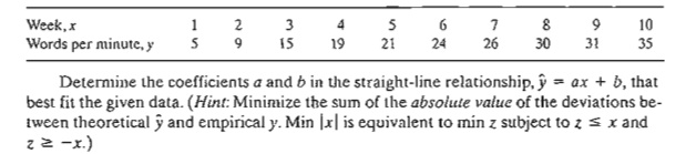
7. Filling a Straight Line into Empirical Data (Regression). In a lO-week typing class for be-ginners, the average speed per student (in words per minute) as a function of the number of weeks in class is given in the following table.

8. Leveling the Terrain for a New Highway. (Stark and Nicholes, 1972) The Arkansas Highway Department is planning a new 10-mile highway on uneven terrain as shown by the profile in Figure 2.10. The width of the construction terrain is approximately 50 yards. To simplify the situation, the terrain profile can be replaced by a step function as shown in the figure. Using heavy machinery, earth removed from high terrain is hauled to fill low areas. There are also two burrow pits, I and II, located at the ends of the lO-mile stretch from which additional earth can be hauled, if needed. Pit I has a capacity of 20,000 cubic yards and pit II a capacity of 15,000 cubic yards. The costs of removing earth from pits I and II are, respectively, $1.50 and $1.90 per cubic yard. The transportation cost per cubic yard per mile is $.15 and the cost of using heavy machinery to load hauling trucks is $.20 per cubic yard. This means that a

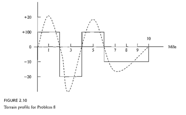
cubic yard from pit I hauled one mile will cost a total of (1.5 + .20) + 1 X .15 = $1.85 and a cubic yard hauled one mile from a hill to a fill area will cost .20 + 1 x .15 = $.35. Devel-op a minimum cost plan for leveling the lO-mile stretch.

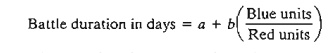
9. Military Planning. (Shepard and Associates, 1988) The Red Army (R) is trying to invade the territory defended by the Blue Army (B). Blue has three defense lines and 200 regular combat units and can draw also on a reserve pool of 200 units. Red plans to attack on two fronts, north and south, and Blue has set up three east-west defense lines, I, II, and III. The purpose of defense lines I and II is to delay the Red Army attack by at least 4 days in each line and to maximize the total duration of the battle. 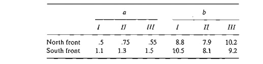The advance time of the Red Army is estimated by the following empirical formula:

The constants a and b are a function of the defense line and the north/south front as the following table shows:

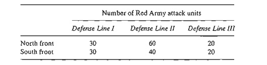
The Blue Army reserve units can be used in defense lines II and II only. The alloca-tion of units by the Red Army to the three defense lines is given in the following table.

How should Blue allocate its resources among the three defense lines and the north/south fronts?

 10. Water Quality Management. (Stark and Nicholes, 1972) Four cities discharge waste water into the same stream. City 1 is upstream, followed downstream by city 2, then city 3, then city 4. Measured alongside the stream, the cities are approximately 15 miles apart. A measure of the amount of pollutants in waste water is the BOD (biochemical oxygen de-mand), which is the weight of oxygen required to stabilize the waste constituent in water. A higher BOD indicates worse water quality. The Environmental Protection Agency (EPA) sets a maximum allowable BOD loading, expressed in lb BOD per gallon. The re-moval of pollutants from waste water takes place in two forms: (1) natural decomposition activity stimulated by the oxygen in the air, and (2) treatment plants at the points of dis-charge before the waste reaches the stream. The objective is to determine the most economical efficiency of each of the four plants that will reduce BOD to acceptable levels. The maximum possible plant efficiency is 99%.

To demonstrate the computations involved in the process, consider the following de-finitions for plant 1:

Q₁ = Stream flow (gal/hour) on the 15-mile reach 1-2 leading to city 2

P₁  = BOD discharge rate (in lb/hr)

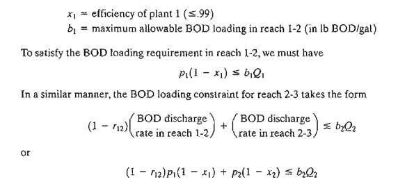
The coefficient r₁₂ (<1) represents the fraction of waste removed in reach 1-2 by decom-position. For reach 2-3, the constraint is

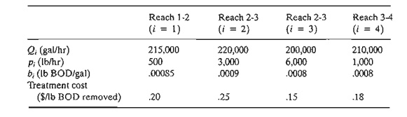
Determine the most economical efficiency for the four plants using the following data (the fraction of BOD removed by decomposition is 6% for all four reaches):

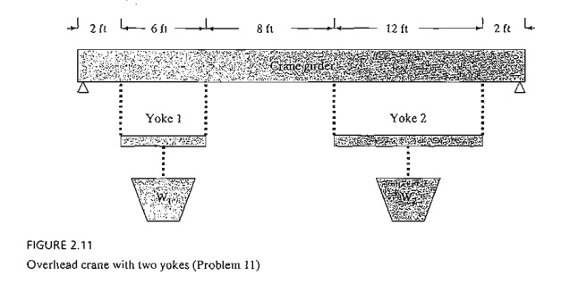
11. Loading Structure. (Stark and Nicholes, 1972) The overhead crane with two lifting yokes in Figure 2.11 is used to transport mixed concrete to a yard for casting concrete barriers.

The concrete bucket hangs at midpoint from the yoke. The crane end rails can support a maximum of 25 kip each and the yoke cables have a 20-kip capacity each. Determine the maximum load capacity, W₁ and W₂. (Hint: At equilibrium, the sum of moments about any point on the girder or yoke is zero.)

12. Allocation of Aircraft to Routes. Consider the problem of assigning aircraft to four routes according to the following data:

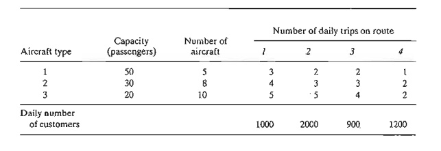
The associated costs, including the penalties for losing customers because of space unavailability, are

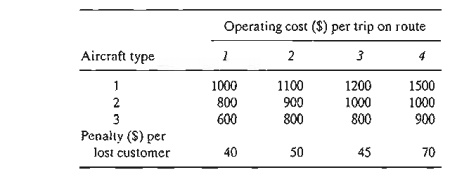
Determine the optimum allocation of aircraft to routes and determine the associated number of trips.