Chapter: Modern Analytical Chemistry: Developing a Standard Method
Searching Algorithms for Response Surfaces
Searching Algorithms for Response Surfaces
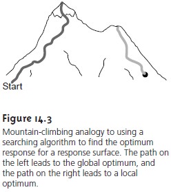
Imagine that you wish to climb to the top of a mountain. Because
the mountain is covered with trees that
obscure its shape,
the shortest path
to the summit
is un- known. Nevertheless, you can reach
the summit by always walking
in a direction that moves you to a higher elevation. The route followed
(Figure 14.3) is the result of a systematic search
for the summit.
Of course, many routes are possible leading from the initial starting point to the
summit. The route
taken, therefore, is deter-
mined by the set of rules (the
algorithm) used to determine the
direction of each step. For example, one algorithm for climbing a mountain is to always
move in the direction that has the steepest slope.
A systematic searching algorithm can also
be used to locate the
optimum re- sponse for an analytical method. To find the optimum
response, we select an initial set of factor levels
and measure the
response. We then
apply the rules
of the search- ing algorithm to determine the next set of factor
levels. This process
is repeated until the algorithm indicates that we have reached the optimum response. Two common searching algorithms are described in this section. First, however, we must
consider how to evaluate a searching algorithm.
Effectiveness and Efficiency
A searching algorithm is characterized by its effec- tiveness and its efficiency. To be effective, the experimentally determined optimum should closely coincide
with the system’s
true optimum. A searching algorithm may fail to find the true optimum for several reasons,
including a poorly
designed algo- rithm, uncertainty in measuring the response, and the presence
of local optima.
A poorly designed algorithm may prematurely end the search.
For example, an algo-
rithm for climbing a mountain
that allows movement
to the north, south, east,
or west will fail to find a summit that can only be reached by moving to the northwest.
When measuring the response is subject to relatively large
random errors, or noise, a spuriously high response may produce a false optimum
from which the searching algorithm cannot move. When
climbing a mountain, boulders encoun- tered
along the way
are examples of “noise” that
must be avoided
if the true
opti- mum is to be found.
The effect of noise can be minimized by increasing the size of the
individual steps such that the change in response is larger than the noise.
Finally, a response
surface may contain
several local optima,
only one of which
is the system’s true, or global, optimum.
This is a problem because
a set of initial
conditions near a local optimum
may be unable
to move toward
the global opti- mum. The mountain shown in Figure 14.3, for example, contains
two peaks, with the
peak on the left being
the true summit.
A search for the summit
beginning at the position
identified by the dot may find the local peak instead of the true sum-
mit. Ideally, a searching algorithm should reach the global optimum
regardless of the initial
set of factor levels. One way to evaluate a searching algorithm’s effective- ness, therefore, is to use several sets of initial
factor levels, finding
the optimum re- sponse for each, and comparing the results.
A second desirable characteristic for a searching algorithm is efficiency. An effi-
cient algorithm moves
from the initial
set of factor
levels to the
optimum response in as few steps as possible.
The rate at which the optimum is approached can be in- creased by taking larger
steps. If the
step size is too large,
however, the difference between the
experimental optimum and
the true optimum
may be unacceptably large. One solution is to adjust the step size during the search,
using larger steps at
the beginning, and
smaller steps as the optimum
response is approached.
One-Factor-at-a-Time Optimization
One
approach to optimizing the quantitative
method for vanadium described earlier
is to select initial concentrations for H2O2 and H2SO4 and measure the
absorbance. We then
increase or decrease the concentration
of one reagent in steps,
while the second
reagent’s concentration remains
constant, until the absorbance decreases in value.
The concentration of the second
reagent is then adjusted until
a decrease in absorbance is again observed. This process
can be stopped after one cycle or repeated until the absorbance reaches a maximum value
or exceeds an acceptable threshold value.
A one-factor-at-a-time optimization is consistent with a commonly held belief that to determine the influ- ence of one factor it is necessary to hold constant all other factors. This is an effective, although not necessarily an ef- ficient, experimental design when the factors are independent. Two factors are considered independent when changing the level of one factor does not influence the effect of changing the other factor’s level. Table 14.1 provides an example of two in- dependent factors.
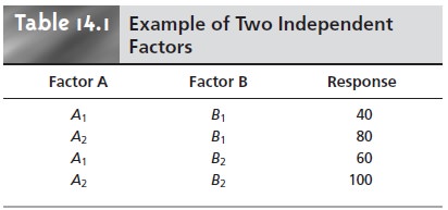
When factor
B is held at level
B1, changing
factor A from level A1
to level A2 increases the response from 40 to 80; thus,
the change in response, ∆R, is
∆R = 80– 40= 40
In the same manner, when factor B is at level B2, we find that
∆R = 100– 60= 40
when the level of factor A changes
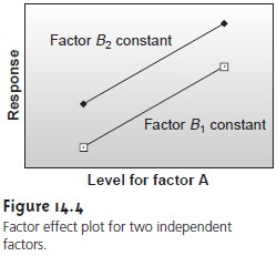
from A1 to A2. We can see this independence graphically by plotting the response versus
the factor levels
for factor A (Figure 14.4). The parallel lines show
that the level
of factor B does not
influence the effect
on the response of changing factor A. In the same manner, the effect of changing factor B’s
level is independent of the
level of factor
A.
Mathematically, two factors
are independent if they do not appear
in the same term in the algebraic equation
describing the response
surface. For example,
factors A and B are independent when the response, R, is given as
R =
2.0 + 0.12A +
0.48B – 0.03A2 – 0.03B2……………14.1
The resulting response surface for equation 14.1 is shown in
Figure 14.5.
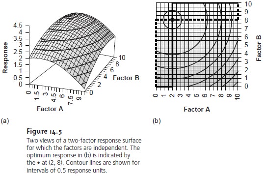
The progress of a searching algorithm is best followed by mapping its path on a
contour plot of the response surface. Positions on the response surface are identified as (a, b)
where a and b are
the levels for factors A and B. Four examples
of a one- factor-at-a-time optimization of the response surface for equation 14.1 are shown
in Figure 14.5b. For those paths
indicated by a solid line,
factor A is optimized first, followed by factor B. The order
of optimization is reversed
for paths marked by a dashed line.
The effectiveness of this
algorithm for optimizing independent factors
is shown by the
fact that the
optimum response at (2, 8) is reached
in a single cycle
from any set
of initial factor
levels. Further- more, it does not matter which
factor is optimized first. Although this algorithm is effective at locating the opti-
mum response, its efficiency is limited by requiring that only a single factor
can be changed
at a time.
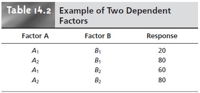
Unfortunately, it is more common to find that two factors are not independent. In Table 14.2,
for instance, changing the level of factor B from level
B1 to level B2 has a significant effect on the response when factor A is at level A1
∆R = 60– 20= 40
but has no effect when factor A is at level A2.
∆R = 80– 80=0
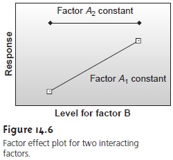
This effect is seen graphically in Figure 14.6. Factors that are not independent are said
to interact. In this case the equation
for the response includes an interaction
term in which both factors
A and B are present.
Equation 14.2, for example, con- tains a final term accounting for the interaction between the factors
A and B.
R =
5.5 + 1.5A +
0.6B – 0.15A2 – 0.0245B2 –
0.0857AB ………..14.2
The resulting response surface for equation 14.2 is shown in
Figure 14.7a.
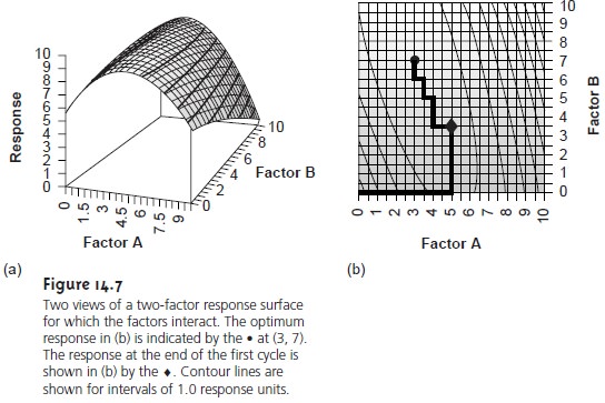
The progress of a one-factor-at-a-time optimization for the
response surface given by equation
14.2 is shown
in Figure 14.7b.
In this case the optimum
response of (3, 7) is not
reached in a single cycle.
If we start at (0,
0), for example, optimizing factor A follows
the solid line
to the point
(5, 0). Optimizing factor B completes the first cycle at the point
(5, 3.5). If our algorithm allows for only a single
cycle, then the optimum
response is not found. The optimum response
usually can be reached
by continuing the search through
additional cycles, as shown in Figure 14.7b.
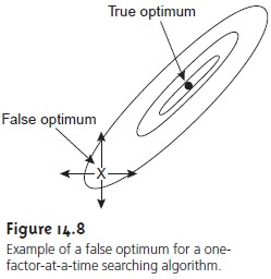
Theefficiency of a one-factor-at-a-time searching algorithm is significantly less whenX the factors interact. An additional
complication with interacting factors is the possi- bility that the search will
end prematurely on a ridge of the response surface, wherea change
in level for
any single factor
results in a smaller response (Figure 14.8).
Simplex Optimization
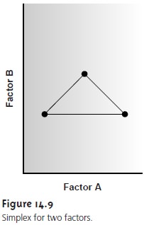
The efficiency of a searching algorithm is improved by al- lowing more than one factor to be changed
at a time. A convenient way to accom- plish this with two factors is to select three sets of initial
factor levels, positioned as the vertices of a triangle (Figure 14.9), and
to measure the
response for each.
The set of factor
levels giving the smallest response
is rejected and replaced with a new set of factor levels using a set of rules. This
process is continued until no further
optimiza- tion is possible. The set of factor levels
is called a simplex. In general, for k factors a simplex is a (k + 1)-dimensional geometric figure.
The initial simplex
is determined by choosing a starting point on the response
surface and selecting step sizes for each factor. Ideally
the step sizes for each factor
should produce an approximately equal change in the response.
For two factors a convenient set
of factor levels
is (a, b), (a +
sA, b), and
(a + 0.5sA, b + 0.87sB), where sA and sB are the step sizes for factors A and B.5 Optimization is achieved using
the following set of rules:
Rule 1. Rank the response for each vertex
of the simplex
from best to worst.
Rule 2. Reject the worst
vertex, and replace
it with a new vertex
generated by reflecting the worst vertex
through the midpoint
of the remaining vertices. The factor levels for the
new vertex are
twice the average
factor levels for
the retained vertices minus
the factor levels
for worst vertex.
Rule 3. If the new
vertex has the
worst response, then
reject the vertex
with the second-worst response, and calculate the new vertex
using rule 2. This rule ensures that the simplex
does not return
to the previous simplex.
Rule 4. Boundary conditions are
a useful way
to limit the
range of possible factor levels. For example,
it may be necessary to limit the concentration of a factor
for solubility reasons
or to limit temperature due to a reagent’s thermal stability. If the new
vertex exceeds a boundary condition, then assign it a
response lower than all other
responses, and follow
rule 3.
Because the size of the simplex remains
constant during the search, this algorithm is called a fixed-sized simplex optimization. Example 14.1 illustrates
the application of these rules.
The fixed-size simplex
searching algorithm is effective at locating the optimum
response for both independent and interacting factors.
Its efficiency, however,
is limited by the simplex’s size.
We can increase its efficiency by allowing the size of the
simplex to expand
or contract in response to the rate
at which the
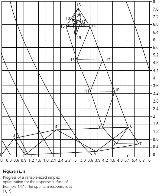
optimum is being approached.3,6 Although the algorithm for a variable-sized simplex is not pre-
sented here, an example of its increased efficiency is shown
Figure 14.11. The
refer- ences and suggested readings may be consulted for
further details.
Related Topics