Mathematical Models of Response Surfaces

Mathematical Models of Response Surfaces

Earlier we noted that a response surface can be described mathematically by an equation relating the response to its factors. If a series of experiments is carried out in which we measure the response for several combinations of factor levels, then lin- ear regression can be used to fit an equation describing the response surface to the data. The calculations for a linear regression when the system is first-order in one factor (a straight line). A complete mathematical treat- ment of linear regression for systems that are second-order or that contain more than one factor is beyond the scope of this text. Nevertheless, the computations for a few special cases are straightforward and are considered in this section.

Theoretical Models of the Response Surface 

Mathematical models for response surfaces are divided into two categories: those based on theory and those that are empirical. Theoretical models are derived from known chemical and physical rela- tionships between the response and the factors. In spectrophotometry, for example, Beer’s law is a theoretical model relating a substance’s absorbance, A, to its concen- tration, C_A

A = εbC_A

where ε is the molar absorptivity, and b is the pathlength of the electromagnetic ra- diation through the sample. A Beer’s law calibration curve, therefore, is a theoretical model of a response surface.

Empirical Models of the Response Surface 

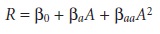
In many cases the underlying theoreti- cal relationship between the response and its factors is unknown, making impossi- ble a theoretical model of the response surface. A model can still be developed if we make some reasonable assumptions about the equation describing the response sur- face. For example, a response surface for two factors, A and B, might be represented by an equation that is first-order in both factors

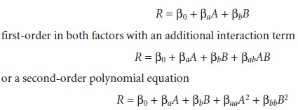
The terms β₀, β_a, β_b, β_ab, β_aa,and β_bb, are adjustable parameters whose values are de- termined by using linear regression to fit the data to the equation. Such equations are empirical models of the response surface because they have no basis in a theo- retical understanding of the relationship between the response and its factors. An empirical model may provide an excellent description of the response surface over a wide range of factor levels. It is more common, however, to find that an empirical model only applies to the range of factor levels for which data have been collected.

To develop an empirical model for a response surface, it is necessary to collect the right data using an appropriate experimental design. Two popular experimental designs are considered in the following sections.

Factorial Designs 

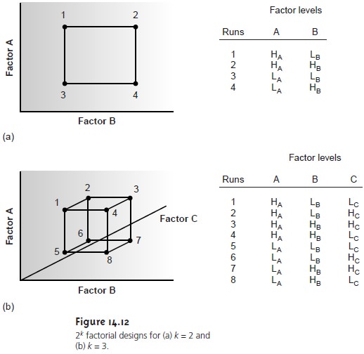
To determine a factor’s effect on the response, it is necessary to measure the response for at least two factor levels. For convenience these levels are labeled high, H_f, and low, L_f, where f is the factor; thus H_A is the high level for factor A, and L_B is the low level for factor B. When more than one factor is included in the empirical model, then each factor’s high level should be paired with both the high and low levels for all other factors. In the same way, the low level for each factor should be paired with the high and low levels for all other factors (Figure 14.12). All together, a minimum of 2k experiments is necessary, where k is the number of fac- tors. This experimental design is known as a 2k factorial design.

The linear regression calculations for a 2k factorial design are straightforward and can be done without the aid of a sophisticated statistical software package. To simplify the computations, factor levels are coded as +1 for the high level, and –1 for the low level. The relationship between a factor’s coded level, x*, and its actual

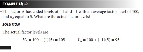
value, x_f, is given as

x_f = c_f + d _fx_f*             …………..14.3

where c_f is the factor’s average level, and d_f is the absolute difference between the factor’s average level and its high and low values. Equation 14.3 is used to transform coded results back to their actual values.

Let’s start by considering a simple example involving two factors, A and B, to which we wish to fit the following empirical model.

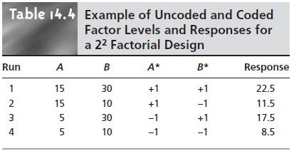
A 2k factorial design with two factors requires four runs, or sets of experimental conditions, for which the uncoded levels, coded levels, and responses are shown in Table 14.4. The terms β₀, β_a, β_b, and β_ab in equation 14.4 account for, respectively, the mean effect (which is the average response), first-order effects due to factors A and B, and the interaction between the two factors. Estimates for these parameters are given by the following equations

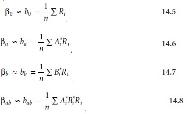
where n is the number of runs, and A* and B* are the coded factor levels for the ithrun. Solving for the estimated parameters using the data in Table 14.4

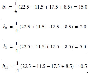
leaves us with the following empirical model for the response surface

R = 15.0 + 2.0A* + 5.0B* + 0.5A*B*              …………..14.9

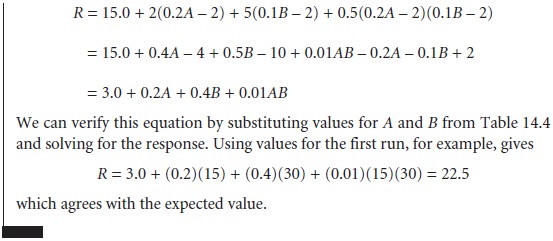
The suitability of this model can be evaluated by substituting values for A* and B* from Table 14.4 and comparing the calculated response to the known response. Using the values for the first run as an example gives

R = 15.0 + (2.0)(+1) + (5.0)(+1) + (0.5)(+1)(+1) = 22.5

which agrees with the known response.

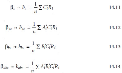
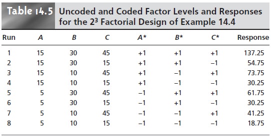
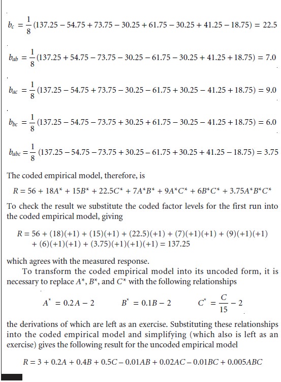
The computation just outlined is easily extended to any number of factors. For a system with three factors, for example, a 23 factorial design can be used to deter- mine the parameters for the empirical model described by the following equation

where A, B, and C are the factors. The terms β₀, β_a, β_b and β_ab are estimated using equations 14.6–14.9. The remaining parameters are estimated using the following equations.

A 2k factorial design is limited to models that include only a factor’s first-order effects on the response. Thus, for a 22 factorial design, it is possible to determine the first-order effect for each factor (β_a and β_b), as well as the interaction between the factors (β_ab). There is insufficient information in the factorial design, however, to determine any higher order effects or interactions. 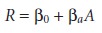This limitation is a consequence of having only two levels for each factor. Consider, for example, a system in which the response is a function of a single factor. Figure 14.13a shows the experimentally measured response for a 21 factorial design in which only two levels of the factor are used. The only empirical model that can be fit to the data is that for a straight line.

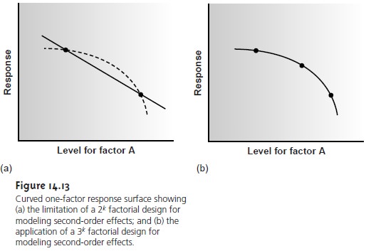
If the actual response is that represented by the dashed curve, then the empirical model is in error. To fit an empirical model that includes curvature, a minimum of three levels must be included for each factor. The 31 factorial design shown in Fig- ure 14.13b, for example, can be fit to an empirical model that includes second-order effects for the factor.

In general, an n-level factorial design can include single-factor and interaction terms up to the (n – 1)th order.

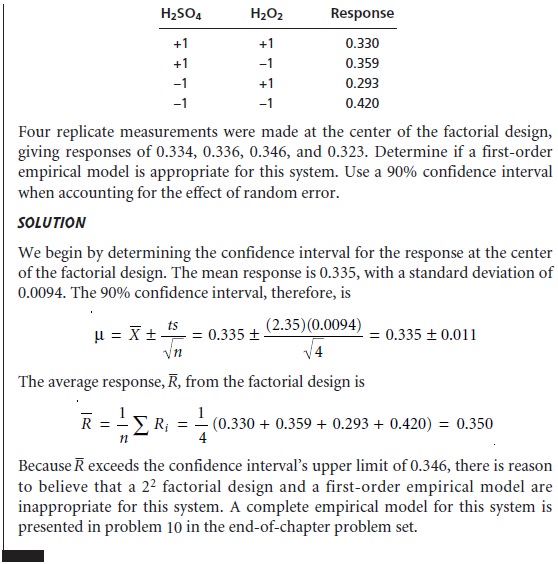
The effectiveness of a first-order empirical model can be judged by measuring the response at the center of the factorial design. If there are no higher order effects, the average response of the runs in a 2k factorial design should be equal to the mea- sured response at the center of the factorial design. The influence of random error can be accounted for by making several determinations of the response at the center of the factorial design and establishing a suitable confidence interval. If the differ- ence between the two responses is significant, then a first-order empirical model is probably not appropriate.

Many systems that cannot be represented by a first-order empirical model can be described by a full second-order polynomial equation, such as that for two factors.

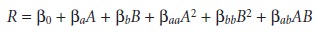
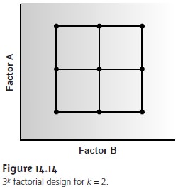
Because each factor must be measured for at least three levels, a convenient experi- mental design is a 3k factorial design. A 32 factorial design for two factors, for exam- ple, is shown in Figure 14.14. The computations for 3k factorial designs are not as easily generalized as those for a 2k factorial design and are not considered in this text.

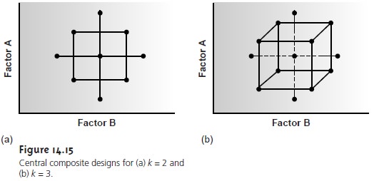
Central Composite Designs 

One limitation to a 3k factorial design is the number of trials that must be run. For two factors, as shown in Figure 14.14, a total of nine trials is needed. This number increases to 27 for three factors and 81 for four factors. A more efficient experimental design for systems containing more than two factors is the central composite design, two examples of which are shown in Figure 14.15. The central composite design consists of a 2k factorial de- sign, which provides data for estimating the first-order effects for each factor and interactions between the factors, and a “star” design consisting of 2k + 1 points, which provides data for estimating second-order effect. Although a central com- posite design for two factors requires the same number of trials, 9, as a 32 facto- rial design, it requires only 15 trials and 25 trials, respectively, for systems involving three or four factors. A discussion of central composite designs, includ- ing computational considerations.