Collaborative Testing and Analysis of Variance

Collaborative Testing and Analysis of Variance

In the two-sample collaborative test, each analyst performs a single determina- tion on two separate samples. The resulting data are reduced to a set of differ- ences, D, and a set of totals, T, each characterized by a mean value and a stan- dard deviation. Extracting values for random errors affecting precision and systematic differences between analysts is relatively straightforward for this ex- perimental design.

An alternative approach for collaborative testing is to have each analyst per- form several replicate determinations on a single, common sample. This approach generates a separate data set for each analyst, requiring a different statistical treat- ment to arrive at estimates for σ_rand and σ_sys.

A variety of statistical methods may be used to compare three or more sets of data. The most commonly used method is an analysis of variance (ANOVA). In its simplest form, a one-way ANOVA allows the importance of a single variable, such as the identity of the analyst, to be determined. The importance of this variable is evaluated by comparing its variance with the variance explained by indeterminate sources of error inherent to the analytical method.

Variance was introduced  as one measure of a data set’s spread around its central tendency. In the context of an analysis of variance, it is useful to see that variance is simply a ratio of the sum of squares for the differences between individual values and their mean, to the degrees of freedom. For example, the vari- ance, s2, of a data set consisting of n measurements is given as

where X_i is the value of a single measurement, and X– is the mean. As we will see, the ability to partition the variance into separate terms for the sum of squares and the degrees of freedom greatly simplifies the calculations in a one-way ANOVA.

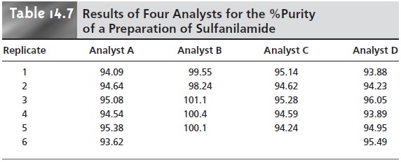
Let’s use a simple example to develop the rationale behind a one-way ANOVA calculation. The data in Table 14.7 show the results obtained by several analysts in de- termining the purity of a single pharmaceutical preparation of sulfanilamide. Each column in this table lists the results obtained by an individual analyst. For conve- nience, entries in the table are represented by the symbol X_ij, where i identifies the an- alyst and j indicates the replicate number; thus X_3,5 is the fifth replicate for the third analyst (and is equal to 94.24%). The variability in the results shown in Table 14.7 arises from two sources: indeterminate errors associated with the analytical procedure that are experienced equally by all analysts, and systematic or determinate errors in- troduced by the analysts.

One way to view the data in Table 14.7 is to treat it as a single system, charac-terized by a global mean, X–, and a global variance, s^2’’ . These parameters are calcu- lated using the following equations.

where h is the total number of samples (in this case the number of analysts), n_i is the number of replicates for the ith sample (in this case the ith analyst), and N is the total number of data points in the system. The global variance provides a measure of the combined influence of indeterminate and systematic errors.

A second way to work with the data in Table 14.7 is to treat the results for each analyst separately. Because the repeatability for any analyst is influenced by indeter- minate errors, the variance, s_w2, of the data in each column provides an estimate of σ²_rand. A better estimate is obtained by pooling the individual variances. The result, rand

which is called the within-sample variance (s_w2 ), is calculated by summing the squares of the differences between the replicates for each sample and that sample’s mean, and dividing by the degrees of freedom.

Finally, the data for each analyst can be reduced to separate mean values, X–_i.

The variance of the individual means about the global mean is called the between- sample variance, s_b2, and is calculated as

where n_i is the number of replicates for the ith sample. The between-sample vari- ance includes contributions from both random and systematic errors and, therefore, provides an estimate for both σ²_rand and σ²_rand.

where n– is approximated as the average number of replicates per analyst.

In a one-way ANOVA of the data in Table 14.7, the null hypothesis is that no significant differences exist between the mean values for each analyst. The alterna- tive hypothesis is that at least one of the means is significantly different. If the null hypothesis is true, then σ²_sys must be zero. Thus, from equations 14.22 and 14.24 both s_w² and s_b² are predictors of σ²_rand and should have similar values. If s_b² is signifi- cantly greater than s_w², then σ²_sys is greater than zero. In this case the alternative hy-pothesis must be accepted, and a significant difference between the means for the analysts has been demonstrated. The test statistic is the F-ratio

which is compared with the critical value F(α, h – 1, N – h). This is a one-tailed signifi- cance test because we are only interested in whether s_b² is significantly greater than s_w².

Both s_b² and s_w² are easy to determine for small data sets. For larger data sets, however, calculating s_w² becomes tedious.* Its calculation is simplified by taking advantage of the relationship between the sum-of-squares terms for the global variance, the within-sample variance, and the between-sample variance. The numerator of equation 14.21, which also is known as the total sum of squares, SS_t, can be split into two terms

SS_t = SS_w + SS_b

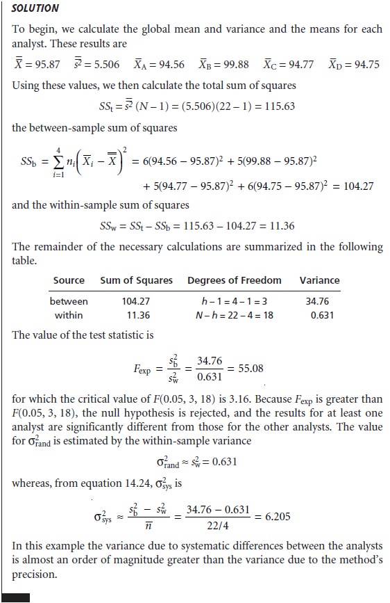
where the sum of squares for the variation within the sample, SS_w, is the numerator of equation 14.22, and the sum of squares between the sample, SS_b, is the numera- tor of equation 14.23. Calculating SS_t and SS_b gives SSw by difference. Dividing SSw and SS_b by their respective degrees of freedom gives s_w² and s_w². Table 14.8 summa- rizes all the necessary equations for a one-way ANOVA calculation. The application of a one-way ANOVA is outlined in Example 14.9.

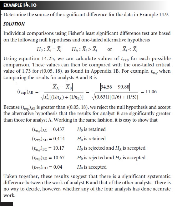
Once a significant difference has been demonstrated by an analysis of variance, a modified version of the t-test, known as Fisher’s least significant difference, can be used to determine which analyst or analysts are responsible for the difference.

The test statistic for comparing the mean values X–₁ and X–₂ is the t-test, except that s_pool is replaced by the square root of the within-sample vari- ance obtained from an analysis of variance.

This value of t_exp is compared with the critical value for t(α, v), where the signifi- cance level is the same as that used in the ANOVA calculation, and the degrees of freedom is the same as that for the within-sample variance. Because we are inter- ested in whether the larger of the two means is significantly greater than the other mean, the value of t(α, v) is that for a one-tail significance test.

An analysis of variance can be extended to systems involving more than a single variable. For example, a two-way ANOVA can be used in a collaborative study to determine the importance to an analytical method of both the analyst and the in- strumentation used. The treatment of multivariable ANOVA is beyond the scope of this text.