Recommendations for Criteria of Rejecting an Observation

RECOMMENDATIONS FOR CRITERIA OF REJECTING AN OBSERVATION

An analyst, while carrying out a series of measurements, invariably comes across with ONE specific result in a set of replicates that obviously appears to be quite ‘out of place’ with the others, and at this juncture he should take an appropriate decision whether to discard (or expunge) this result from any further consideration. Thus, two situations often arise, namely :

(i) Number of replicates being small, and

(ii) Number of replicates being large.

A. Number of Replicates being Small

An analyst in the true sense encounters a serious problem when the number of replicates at his disposal is SMALL. Firstly, the divergent result shows a distinct and significant effect upon the mean value ( x’) ; and secondly, the prevailing scanty available data does not permit getting at the real statistical analysis of the status of the suspected result.

B. Number of Replicates being Large

In this instance, the analyst has the privilege of rejecting one value (i.e., the ‘out-of place’ value) as it is not an important one by virtue of the following two main reasons :

Firstly, a single value shall exert merely a small effect upon the mean value ( x ) ; and secondly, the treatment of data with the real statistical analysis would certainly reveal vividly the probability that the suspected ‘out of place’ result is a bonafide member of the same population as the others.

Blaedel et al.* (1951), Wilson** (1952) and Laitinen*** (1960) have put forward more broadly accepted and recommended criteria of rejecting an observation.

1. Rules Based on the Average Deviation

Both ‘2.5d’ and ‘4d’ rules are quite familiar to analysts. They may be applied in a sequential manner as follows :

(i) Calculate the mean ( x’ ) and average deviation ( d’ ) of the ‘good’ results,

(ii) Determine the deviation of the ‘suspected’ result from the mean of the ‘good’ results,

(iii) In case, the deviation of the suspected result was found to be either 2.5 times the average deviation of the good results (i.e., ‘2.5d’ rule) or 4 times the average deviation of the good results (i.e.‘4d’ rule) the suspected result was rejected out right ; otherwise the result was duly retained.

Note : The ‘limit for rejection’ seems to be too low for both the said rules.

2. Rules Based on the Range

The Q test, suggested by Dean and Dixon**** (1951) is statistically correct and valid, and it may be applied easily as stated below :

(i) Calculate the range of the results,

(ii) Determine the difference between the suspected result and its closest neighbour,

(iii) Divide the difference obtained in (ii) above by the range from (i) to arrive at the rejection Quotient Q,

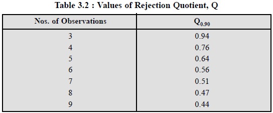
(iv) Finally, consult a table of Q-values. In case, the computed value of Q is found to be greater than the value given in the table, the result in question can be rejected outright with 90% confidence that it was perhaps subject to some factor or the other which never affected the other results.

Table 3.2, records some of the Q-values as given below :

Example : Five determinations of the ampicillin content in capsules of a marketed product gave the following results : 0.248, 0.245, 0.265, 0.249 and 0.250 mg per capsule. Apply the Q-test to find out if the 0.265 value can be rejected.

The value of Q is :

The value in Table 3.2, at n = 5 is Q = 0.64. Because, the determined value 0.75 > 0.64, according to ‘rule based on the range’ the result i.e., 0.265 can be rejected.

Note : The Q-test administers excellent justification for the outright rejection of abnormally erroneous values ; however, it fails to eliminate the problem with less deviant suspicious values.