Chapter: Pharmaceutical Drug Analysis: Errors In Pharmaceutical Analysis and Statistical Validation
Method of Least Squares
METHOD OF LEAST SQUARES
A number of pharmaceutical analytical methods are solely
based on instrumental measurements of an absolutely physical nature, such as :
measuring peak areas with the help of a gas-chromatograph (GC), and measuring
absorbance of a solution using a spectrophotometer (UV). In both these
instances, the physical characteristics are directly proportional to the
concentration of the analyte under examination. In usual prac-tice, a number of
solutions having known concentrations is prepared and the response of the
instrument is subsequently measured for each standard solution. Finally, a
standard curve or calibration curve is plotted between the observed response Vs concentration, which invariably gives
rise to straight line. It has been noticed, that the experimental points rarely
fall exactly upon a straight line by virtue of the indeterminate errors caused
by the instrument readings. At this juncture, an analyst is confronted with the
tedious problem to obtain the ‘best’ straight line for the standard curve based
on the observed points so that the error in estimating the concentration of the
unknown sample is brought down to the least possible extent. At this stage,
instead of deciding to draw the line merely on an analyst’s judgement,
statistics comes to the rescue by providing a mathematical relationship whereby
the analyst not only may calculate the slope objectively but also can obtain
the ‘best’ straight line. The statistical process involved is termed as the
method of least squares.
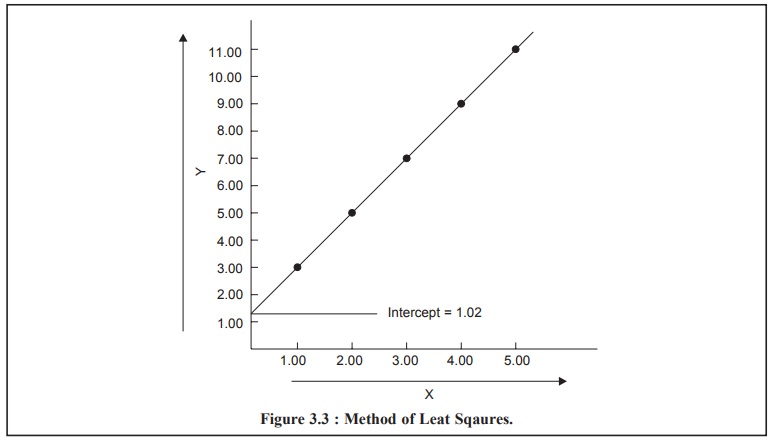
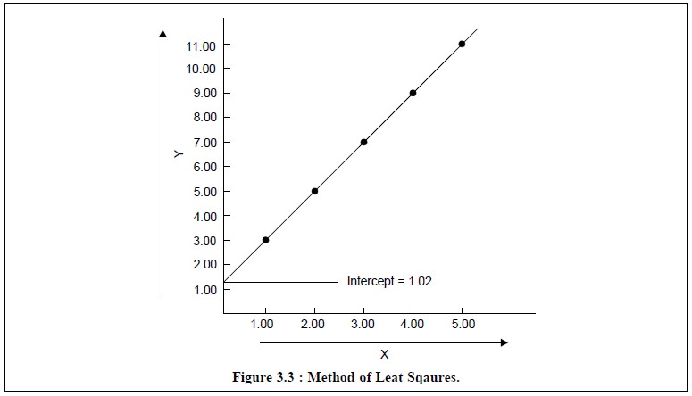
Example : The results obtained from the
determination of concentration of the standard solutions and measurements
of corresponding peak areas with a GC are recorded in Table 3.1 and plotted in
Figure 3.3 ; where the former is represented along the x-axis and the latter along the y-axis.
How to draw the’ ‘best’ straight line through all these points ?
Considering that the relationship between the
concentration and the observed peak areas is a linear one, the equation for a
straight line may be expressed as :
y = mx + b
where, m = Slope of the line, and
b = Intercept on the y-axis.
It may also be assumed that values of x are free of any error.
Presumably, the indeterminate errors caused by the
instrument readings, y, are
responsible for not allowing the ‘data points’ to fall exactly on the line.
Therefore, the sum of the squares of the deviations obtained from the real
instrument readings with respect to the correct values are minimized
coinsiderably by adjusting adequately the values of the slope, m, and the intercept, b.
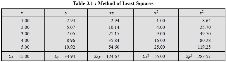
Table 3.1, comprises the values of x and y to enable plot of
the graph in Figure 3.3, besides values of x2, y2 and xy and also the sums
of all these terms.
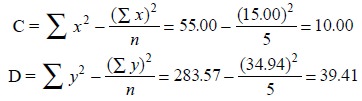
Statistically, the slope (m) and intercept (b) of
the straight line may be obtained by the help of the following equations :
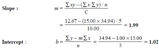
Therefore, the equation of the line is
y = 1.99x + 1.02
Thus, the standard deviation of the y values, Sy, is given by
:
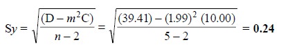
The number of degrees of freedom in the above expression
is n – 2, because two degrees have
already been consumed while calculating the values of m and b earlier.
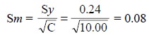
The standard deviation of the slope, Sm, is given by :
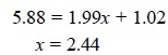
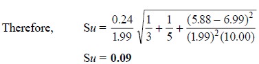
At this point, let us suppose that the ‘calibration
curve’ is used to find out the concentration of the ‘unknown’. Assuming that
three determinations have been carried out separately, thereby giving three y values of 5.85, 5.88, 5.91, or an
average value, yu , of
5.88. Thus, using the expression : y
= mx + b, we have
The standard deviation (Su) in this result is obtained from the expression :
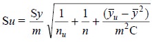
where, nu = Number of
determination of unknown,
n = Number of points in the
calibration graph, and
y’ = Average of the y-values
in the calibration graph (i.e.,
34.94/5 = 6.99)
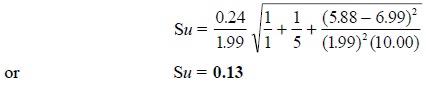
In case, the above statistical analysis has been based on
a single determination, for instance : y
= 5.88, the value of Su shall come
out to be :
Related Topics