Chapter: 12th Maths : UNIT 9 : Applications of Integration
Fundamental Theorems of Integral Calculus and their Applications
Fundamental Theorems of Integral Calculus and their Applications
We observe in the above examples that evaluation of bŌł½af ( x)dx as a limit of the sum is quite tedious, even if f ( x) is a very simple function. Both Newton and Leibnitz, more or less at the same time, devised an easy method for evaluating definite integrals. Their method is based upon two celebrated theorems known as First Fundamental Theorem and Second Fundamental Theorem of Integral Calculus. These theorems establish the connection between a function and its anti-derivative (if it exists). In fact, the two theorems provide a link between differential calculus and integral calculus. We state below the above important theorems without proofs.
Theorem 9.1 (First Fundamental Theorem of Integral Calculus)
If f ( x) be a continuous function defined on a closed interval [a , b] and F (x) = xŌł½a f (u)du, a < x < b then, d/dx F (x) = f ( x). In other words, F ( x) is an anti-derivative of f ( x).
Theorem 9.2 (Second Fundamental Theorem of Integral Calculus)
If f ( x) be a continuous function defined on a closed interval [a , b] and F ( x) is an anti derivative of f ( x), then,
bfa ( x)dx = F (b) ŌłÆ F ( a).
Note
Since F (b) ŌłÆ F ( a) is the value of the definite integral (Riemann integral) bŌł½a f ( x)dx, any arbitrary constant added to the anti-derivative F ( x) cancels out and hence it is not necessary to add an arbitrary constant to the anti-derivative, when we are evaluating definite integrals. As a short-hand form, we write F (b) ŌłÆ F ( a) = [ F ( x)]ba . The value of a definite integral is unique.
By the second fundamental theorem of integral calculus, the following properties of definite integrals hold. They are stated here without proof.

i.e., definite integral is independent of the change of variable.

i.e., the value of the definite integral changes by minus sign if the limits are interchanged.

This property is used for evaluating definite integrals by making substitution.
We illustrate the use of the above properties by the following examples.


Example 9.14
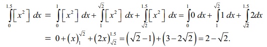
Evaluate : 1.5Ōł½0 [x2] dx, where [ x] is the greatest integer function.
Solution
We know that the greatest integer function [ x] is the largest integer less than or equal to x. In other words, it is defined by [ x ] = n , if n Ōēż x < (n +1) , where n is an integer.

We note that the above function is not continuous on [0,1.5] .
But, it is continuous in each of the sub-intervals [0,1) , [1, ŌłÜ2 ) and [ ŌłÜ2,1.5] ; that is, it is piece-wise continuous on [0,1.5] .
See Fig. 9.6. Hence, we get

Next, we give examples to illustrate the application of Property 5.


We derive some more properties of definite integrals.
Property 6

bŌł½a f ( x) dx = bŌł½a f (a +b ŌłÆ x) dx
Proof
Let u = a + b ŌłÆ x . Then, we get dx = ŌłÆdu .
When x = a , u = a + b ŌłÆ a = b . When x = b , we get u = a + b ŌłÆ b = a .
Ōł┤ bŌł½a f ( x)dx = aŌł½b f ( a + b ŌłÆu)(ŌłÆdu) = bŌł½a f ( a + b ŌłÆu)du
= Ōł½ab f ( a + b ŌłÆ x)dx .
Note
Replace a by 0 and b by a in the above property we get the following property
0 Ōł½ a f ( x) dx = Ōł½0a f ( a ŌłÆ x ) dx .

Property 7

Property 8
If f ( x) is an even function, then ŌłÆaŌł½a f ( x) dx = 20Ōł½a f ( x) dx.
(Recall that a function f ( x) is an even function if and only if f (ŌłÆ x ) = f ( x). )
Proof
By property 3, we have
ŌłÆaŌł½a f ( x) dx = ŌłÆaŌł½0 f ( x) dx + 0Ōł½a f ( x) dx .
In the integral 0Ōł½ŌłÆa f ( x) dx , let us make the substitution, x = ŌłÆu. Then, dx = ŌłÆdu.
When x = ŌłÆa , we get u = a , when x = 0 , we get u = 0 , So, we get
ŌłÆaŌł½0 f ( x) dx = 0Ōł½a f ( ŌłÆ u)( ŌłÆdu) = 0Ōł½a f ( ŌłÆu) du = 0Ōł½a f ( ŌłÆ x) dx = 0Ōł½a f ( x) dx . ... (2)
Substituting equation (2) in equation (1), we get
ŌłÆaŌł½a f ( x) dx = 0Ōł½a f (x) dx + 0Ōł½a f (x) dx = 20Ōł½a f (x) dx .
Property 9
If f ( x) is an odd function, then ŌłÆaŌł½a f ( x) dx = 0.
(Recall that a function f ( x) is an odd function if and only if f (ŌłÆ x ) = ŌłÆ f ( x). )
Proof
By property 3, we have
ŌłÆa Ōł½a f ( x) dx = ŌłÆa Ōł½ 0f ( x) dx + 0Ōł½a f ( x) dx .
Consider ŌłÆaŌł½0 f ( x) dx . In this integral, let us make the substitution, x = ŌłÆu. Then, dx = ŌłÆdu.
When x = ŌłÆa , we get u = a ; when x = 0 , we get u = 0 . So, we get
ŌłÆaŌł½0 f ( x) dx = a Ōł½0 f ( ŌłÆ u)( ŌłÆdu) = aŌł½0 f ( ŌłÆu) du = a Ōł½0 f ( ŌłÆ x) dx = ŌłÆ a Ōł½0 f ( x) dx . ... (2)
Substituting equation (2) in equation (1), we get
aŌł½ŌłÆa f ( x) dx = aŌł½0 f ( x) dx ŌłÆ aŌł½0 f ( x) dx = 0
Property 10
If f (2a ŌłÆ x ) = f ( x), then 2aŌł½0 f ( x) dx = 2 aŌł½0 f ( x) dx.
Proof
By property 7, we have
2aŌł½0 f ( x) dx = aŌł½0 [ f ( x) + f ( 2a ŌłÆ x ) ] dx. ...(1)
Setting the condition f (2a ŌłÆ x ) = f (x) in equation (1), we get
0Ōł½2a f (x) dx = aŌł½0 [ f (x ) + f (x)]dx = 2 aŌł½0 f (x) dx.
Property 11
If f ( 2a ŌłÆ x ) = ŌłÆ f ( x), then 2aŌł½0 ( x) dx = 0.
Proof
By property 7, we have
2a Ōł½0 f ( x) dx = aŌł½0 [ f ( x) + f ( 2a ŌłÆ x ) ]dx. ... (1)
Setting the condition f (2a ŌłÆ x ) = ŌłÆ f (x) in equation (1), we get
2aŌł½0 f ( x) dx = Ōł½0a [ f ( x ) ŌłÆ f ( x)]dx = 0.
Property 12
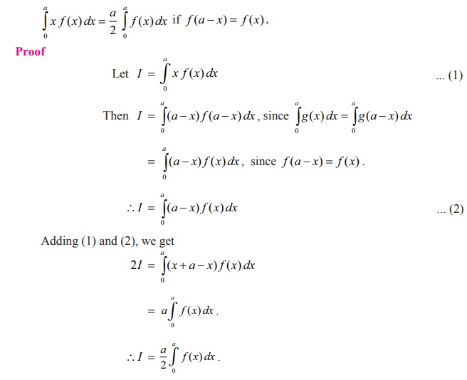
Note
This property help us to remove the factor x present in the integrand of the LHS.
Example 9.20
Show that  , where g (sin x) is a function of sin x .
Solution
We know that
2aŌł½0 f ( x) dx = 2 aŌł½0 f ( x) dx if f (2a ŌłÆ x ) = f (x) .
Take 2a = ŽĆ and f (x) = g (sin x) .
Then, f (2a ŌłÆ x) = g (sin(ŽĆ ŌłÆ x)) = g (sin x) = f (x) .
Ōł┤Ōł½02a f (x) dx = 2Ōł½0a f (x) dx .

Result
Note
The above result is useful in evaluating definite integrals of the type ŽĆŌł½0 g (sin x) dx .
Example 9.21

Example 9.22
Show that 2ŽĆŌł½0 g (cos x) dx =20Ōł½ŽĆ g (cos x) dx , where g (cos x) is a function of cos x .
Solution
Take 2a = 2ŽĆ and f (x) = g (cos x) .
Then, f (2a ŌłÆ x) = f (2ŽĆ ŌłÆ x) = g (cos(2ŽĆ ŌłÆ x)) = g (cos x) = f (x)
Ōł┤ 2aŌł½0 f (x) dx = 2 aŌł½0 f (x) dx .
Ōł┤ 2aŌł½0 g (cos x) dx = 2 ŽĆŌł½0 g (cos x) dx .
Result
2ŽĆŌł½0 g (cos x) dx =2 ŽĆŌł½0 g (cos x) dx.
Note
The above result is useful in evaluating definite integrals of the type 2ŽĆŌł½0 g (cos x) dx.
Example 9.23
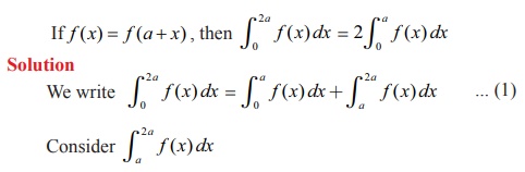
Substituting x = a + u , we have dx = du ; when x = a, u = 0 and when x = 2a, u = a .
Ōł┤2aŌł½a f (x) dx = aŌł½0 f (a + u ) du = aŌł½0 f (u ) du , since f (x) = f (a + x)
= aŌł½0 f (x) dx . ... (2)
Substituting (2) in (1), we get
2aŌł½0 f (x) dx = 2aŌł½0 f (x) dx .
Example 9.24

Solution
Let f(x) = x cos x .Then f(-x) = (ŌłÆ x) cos(ŌłÆ x) = xcos = ŌłÆ f(x).
So f(x) = x cos x is an odd function.
Hence, applying the property, for odd function f(x)


Related Topics