Applications of Integration | Mathematics - Definite Integral as the Limit of a Sum | 12th Maths : UNIT 9 : Applications of Integration
Chapter: 12th Maths : UNIT 9 : Applications of Integration
Definite Integral as the Limit of a Sum
Definite Integral
as the Limit of a Sum
Riemann Integral
Consider
a real-valued, bounded function f (x)
defined on the closed and bounded interval[a,
b ], a < b.
The function f ( x) need not have the same sign on [a , b] ; that is, f ( x)
may have positive as well as negative values on [a , b] . See Fig 9.2.
Partition the interval [a , b] into n subintervals [x0
, x1 ],[x1 , x2 ], ŌĆ” ,[xn
ŌłÆ
2 , xnŌłÆ1 ],[xn ŌłÆ1 , xn ] such that
a = x0 < x1 < x2 < < xn ŌłÆ1 < xn = b.
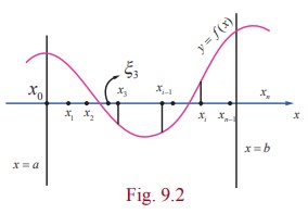
In each
subinterval [xi ŌłÆ1 , xi ], i =
1, 2, ŌĆ”. , n, choose a real number ╬Ši
arbitrarily such that xi ŌłÆ1 Ōēż ╬Ši Ōēż xi.
Consider
the sum Ōłæni=1 f
(╬Ši )( xi ŌłÆ xi
ŌłÆ1 ) = f (╬Š1 )(x1 ŌłÆ x0
) +
f (╬Š2 )(x2 ŌłÆ x1
) + ŌĆ” +
f (╬Šn )(xn ŌłÆ xnŌłÆ1 ) ŌĆ”.(1)
The sum in
(1) is called a Riemann
sum of f ( x) corresponding to the partition [x0 , x1 ],[x1 ,
x2 ], . . . ,[xn ŌłÆ1 ,
xn ] of [a
, b]. Since there are infinitely many values ╬Ši satisfying the condition xi ŌłÆ1 Ōēż ╬Ši Ōēż xi ,
there are infinitely many Riemann sums of f ( x) corresponding to the same partition [x0 , x1 ],[x1 ,
x2 ], . . . ,[xn ŌłÆ1 ,
xn ] of [a
, b]. If, under the limiting process
n ŌåÆ Ōł× and max ( xi ŌłÆ xi ŌłÆ1)ŌåÆ 0, the sum in (1) tends to a finite value, say A, then the value A is called the definite integral of f ( x) with respect to x on [a , b] . It is also
called the Riemann
integral of f ( x) on [a , b] and is denoted by bŌł½a
f ( x)dx and
is read as the integral of f ( x) with respect to x from a to b . If a = b, then we have aŌł½a
f ( x)dx = 0.
Note
In the
present chapter, we consider bounded functions f ( x) that are
continuous on[a , b] . However, the Riemann integral of f ( x)
on [a , b] also exists for bounded functions f ( x) that are piece-wise
continuous on[a , b] .We have used the same symbol Ōł½ both for definite integral
and anti-derivative (indefinite integral). The reason will be clear after we
state the Fundamental Theorems of Integral Calculus. The variable x is dummy in the sense that it is
selected at our choice only. So we can write bŌł½a f (x)dx as bŌł½a f (u)du . So, we have bŌł½a f (x)dx = bŌł½a f (u)du . As max ( xi ŌłÆ xiŌłÆ1) ŌåÆ 0, all the three points xi ŌłÆ1 , ╬Ši , and xi of each subinterval [ xi ŌłÆ1 ,
xi ] are dragged into a single point. We have already indicated
that there are infinitely many ways of choosing the evaluation point ╬Ši in the subinterval [ xi ŌłÆ1 , xi ] , i =
1, 2, . . . , n . By choosing ╬Ši =xi ŌłÆ1 , i = 1, 2, , n , we
have
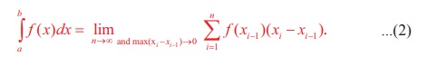
Equation (2) is known as the left-end rule for evaluating the Riemann integral.
By
choosing ╬Ši =xi , i =
1, 2,. . . , n , we have
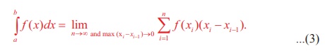
Equation
(3) is known as the right-end rule for evaluating the Riemann
integral.
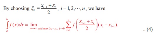
Equation
(4) is known as the mid-point rule for evaluating the Riemann
integral.
Remarks
(1) If
the Riemann integral bŌł½a f ( x)dx exists, then the Riemann integral xŌł½a
f (u)du is a
well-defined
real number for every x Ōłł[a,
b] . So, we can define a function F ( x) on [a , b]
such that F ( x) = xŌł½a f (u)du, x
Ōłł[a,
b] .
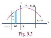
(2) If f (x) Ōēź 0 for all x Ōłł[a,
b] , then the Riemann integral bŌł½af (
x)dx is equal to the geometric
area of the region bounded by the graph of y
=
f ( x) , the x-axis, the
lines x =
a and x = b . See Fig. 9.3.
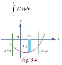
(3) If f (
x) Ōēż 0 for all x Ōłł[a,
b] , then the Riemann integral bŌł½a f ( x)dx is
equal to the negative of the geometric area of the region bounded by the graph
of y = f ( x)
, the x-axis, the lines x = a
and x = b
. See Fig. 9.4. In this case, the geometric area of the region bounded by the
graph of y =
f ( x) , the x-axis, the
lines x =
a and x = b is given by
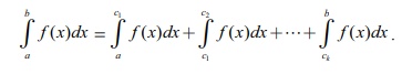
(4) If f (x) takes positive as well as negative
values on [a , b] , then the interval [a , b] can be divided into subintervals
[a , c1 ] , [c1 , c2 ] ,. . . , [ck , b] such that f (x) has the same sign throughout each
of subintervals. So, the Riemann integral bŌł½a f (x)dx is given by
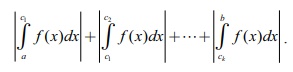
In this
case, the geometric area of the region bounded by the graph of y = f (
x) , the x-axis, the lines x =
a and x = b is given by
For
instance, consider the following graph of a function f ( x), x Ōłł[a,
b] . See Fig. 9.5. Here, A1 , A2 and, A3 denote geometric areas of the
individual parts.
Then,
the definite integral bŌł½a f ( x)dx is given by
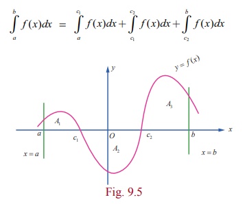
= A1ŌłÆA2+A3.
The
geometric area of the region bounded by the graph of y = f ( x) , the x ŌłÆ axis, the lines x = a and x = b is given by A1 + A2 + A3 . In view of the above discussion,
it is clear that a Riemann integral need not represent geometrical area.
Note
Even if
we do not mention explicitly, it is always understood that the areas are
measured in square units and volumes are measured in cubic units.
Example 9.1
Estimate
the value of Ōł½00.5 x2dx using the Riemann sums corresponding
to 5 subintervals of equal width and applying (i) left-end rule (ii) right-end
rule (iii) the mid-point rule.
Solution
Here a = 0, b = 0.5, n =
5, f (x) = x2
So, the width
of each subinterval is
h
= ╬öx = bŌłÆa / n = 0.5ŌłÆ0 / 5 = 0.1.
The
partition of the interval is given by the points
x0 = 0,
x1 = x0 + h = 0 + 0.1 = 0.1
x2 = x1 + h = 0.1+ 0.1 = 0.2
x3= x2 + h = 0.2 + 0.1 = 0.3
x4= x3 + h = 0.3 + 0.1 = 0.4
x5= x4 + h = 0.4 + 0.1 = 0.5
(i) The
left-end rule for Riemann sum with equal width Δx is
S = [ f(x0) + f (x1) + . .
. + f ( x nŌłÆ1 )╬öx .
S = [f
( 0) + f ( 0.1) + f ( 0.2) + f ( 0.3) + f ( 0.4) ] (0.1)
= [ 0.00 + 0.01+ 0.04 +
0.09 +
0.16] (0.1)
=
0.03
Ōł┤ Ōł½00.5 x2 dx is approximately 0.03 .
(ii) The
right-end rule for Riemann sum with equal width Dx is
S = [ f(x1)
+ f (x2) + . . . + f ( x n )Δx .
S = [
f ( 0.1) + f ( 0.2) + f ( 0.3) + f ( 0.4) + f ( 0.5) ] (0.1)
= [ 0.01+ 0.04 + 0.09 + 0.16 + 0.25](0.1) = 0.055 .
Ōł┤ Ōł½00.5 x2 dx is approximately 0.055 .
(iii) The
mid-point rule for Riemann sum with equal width Δx is
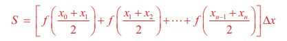
S = [ f ( 0.05) + f ( 0.15) + f ( 0.25) + f ( 0.35) + f ( 0.45) ] (0.1)
= [ 0.0025 + 0.0225 + 0.0625 + 0.1225 + 0.2025](0.1)
= 0.04125 .
Ōł┤ Ōł½00.5 x2dx is approximately 0.04125 .
Related Topics