Two-Sample Collaborative Testing

Two-Sample Collaborative Testing

The design of a collaborative test must provide the additional information needed to separate the effect of random error from that due to systematic errors intro- duced by the analysts. One simple approach, which is accepted by the Association of Official Analytical Chemists, is to have each analyst analyze two samples, X and Y, that are similar in both matrix and concentration of analyte. The results ob- tained by each analyst are plotted as a single point on a two-sample chart, using the result for one sample as the x-coordinate and the value for the other sample as the y-coordinate.8,9

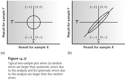
A two-sample chart is divided into four quadrants, identified as (+, +), (–, +), (–, –), and (+, –), depending on whether the points in the quadrant have values for the two samples that are larger or smaller than the mean values for samples X and Y. Thus, the quadrant (+, –) contains all points for which the result for sample X is larger than the mean for sample X, and for which the result for sample Y is less than the mean for sample Y. 

If the variation in results is dominated by random errors, then the points should be distributed randomly in all four quadrants, with an equal number of points in each quadrant. Furthermore, the points will be clustered in a circular pattern whose center is the mean values for the two samples (Figure 14.17a). When systematic errors are significantly larger than random errors, then the points will be found primarily in the (+, +) and (–, –) quadrants and will be clus- tered in an elliptical pattern around a line bisecting these quadrants at a 45° angle (Figure 14.17b).

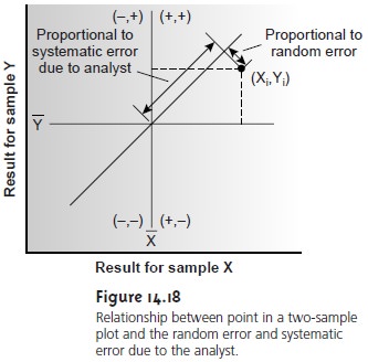
A visual inspection of a two-sample chart provides an effectivemeans for qualitatively evaluating the results obtained by each analyst and of the capabilities of a proposed standard method. If no random errors are present, then all points will be found on the 45° line. The length of a perpendicular line from any point to the 45° line, there- fore, is proportional to the effect of random error on that analyst’s re- sults (Figure 14.18). The distance from the intersection of the lines for the mean values of samples X and Y, to the perpendicular projection of a point on the 45° line, is proportional to the analyst’s systematic error (Figure 14.18). An ideal standard method is characterized by small random errors and small systematic errors due to the analysts and should show a compact clustering of points that is more circular than elliptical.

The data used to construct a two-sample chart can also be used to separate the total variation of the data, σ_tot, into contributions from random error, σ_rand, and systematic errors due to the analysts, σ_sys. Since an analyst’s systematic errors should be present at the same level in the analysis of samples X and Y, the differ- ence, D, between the results for the two samples

D_i = X_i – Y_i

is influenced only by random error. The contribution from random error, there- fore, is estimated by the standard deviation of the differences for each analyst

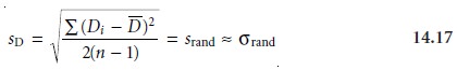
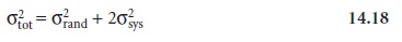
where n is the number of analysts. The inclusion of a factor of 2 in the denominator of equation 14.17 is the result of using two values to determine D_i. The total, T, of each analyst’s results for the two samples

T_i = X_i + Y_i

contains contributions from both random error and twice the analyst’s systematic error; thus

The standard deviation of the totals provides an estimate for σ_tot.

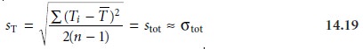
Again, the factor of 2 in the denominator is the result of using two values to deter- mine T_i.

If systematic errors due to the analysts are significantly larger than random er- rors, then s_T should be larger than s_D. This can be tested statistically using a one- tailed F-test

where the degrees of freedom for both the numerator and the denominator are n – 1. If s_T is significantly larger than s_D, then we can use equation 14.18 to separate the data’s total variation into that due to random error and that due to the system- atic errors of the analysts.

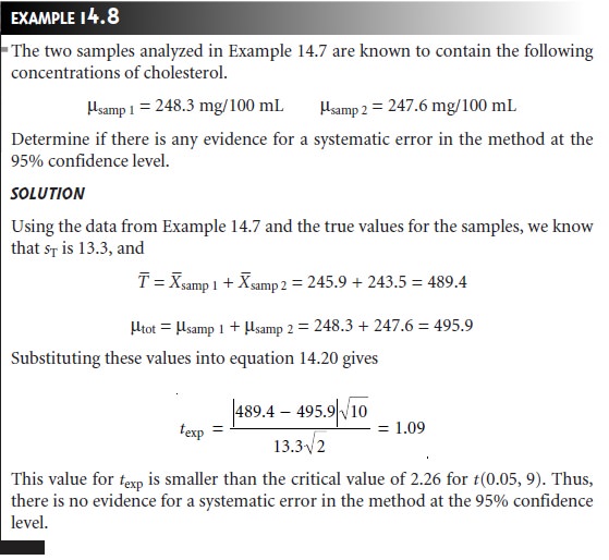
When the true values for the two samples are known, it is possible to test for the presence of systematic errors in the method. If no systematic method errors occur, then the sum of the true values for the samples, μ_tot

μtot = μsamp X + μsamp Y

will fall within the confidence interval around the average value, T’. A two-tailed t-test, with the following null and alternative hypotheses

is used to determine whether there is any evidence for systematic method errors. The test statistic, t_exp, is given as

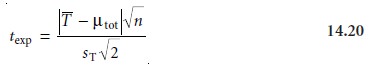
and has n – 1 degrees of freedom. The Rt[2] in the denominator is included because s_T, as given in equation 14.19, underestimates the standard deviation when comparing T’ to μ_tot.

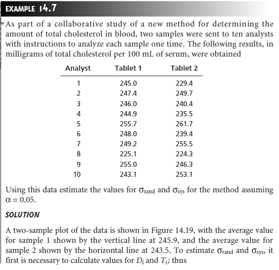
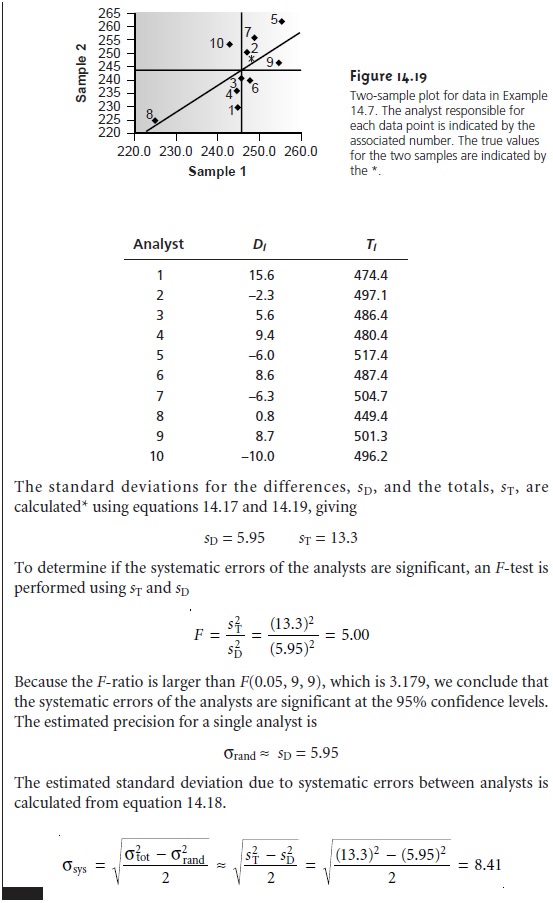
In Examples 14.7 and 14.8 we have seen how a collaborative test using a pair of closely related samples can be used to evaluate a method. Ideally, a collaborative test should involve several pairs of samples, whose concentrations of analyte span the method’s anticipated useful range. In this way the method can be evaluated for con- stant sources of error, and the expected relative standard deviation and bias for dif- ferent levels of analyte can be determined.