Pipelining

Pipelining

1 What is Pipelining?

2 Successive Over-Relaxation (SOR): An Example

3 Fully Permutable Loops

4 Pipelining Fully Permutable Loops

5 General Theory

6 Time-Partition Constraints

7 Solving Time-Partition Constraints by Farkas' Lemma

8 Code Transformations

9 Parallelism With Minimum Synchronization

10 Exercises for Section 11.9

In pipelining, a task is decomposed into a number of stages to be performed on different processors. For example, a task computed using a loop of n iterations can be structured as a pipeline of n stages. Each stage is assigned to a different processor; when one processor is finished with its stage, the results are passed as input to the next processor in the pipeline.

In the following, we start by explaining the concept of pipelining in more detail. We then show a real-life numerical algorithm, known as successive over-relaxation, to illustrate the conditions under which pipelining can be applied, in Section 11.9.2. We then formally define the constraints that need to be solved in Section 11.9.6, and describe an algorithm for solving them in Section 11.9.7. Programs that have multiple independent solutions to the time-partition constraints are known as having outermost fully permutable  loops;  such loops can be pipelined easily, as discussed in Section 11.9.8.

1. What is Pipelining?

Our initial attempts to parallelize loops partitioned the iterations of a loop nest so that two iterations that shared data were assigned to the same processor. Pipelining allows processors to share data, but generally does so only in a "local," way, with data passed from one processor to another that is adjacent in the processor space. Here is a simple example.

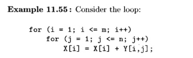
This code sums up the ith row of Y and adds it to the ith element of X. The inner loop, corresponding to the summation, must be performed sequentially

because of the data dependence;6 however, the different summation tasks are independent. We can parallelize this code by having each processor perform a separate summation. Processor i accesses row i of Y and updates the ith element of X.

Alternatively, we can structure the processors to execute the summation in a pipeline, and derive parallelism by overlapping the execution of the summations, as shown in Fig. 11.49. More specifically, each iteration of the inner loop can be treated as a stage of a pipeline: stage j takes an element of X generated in the previous stage, adds to it an element of Y, and passes the result to the next stage. Notice that in this case, each processor accesses a column, instead of a row, of Y. If Y is stored in column-major form, there is a gain in locality by partitioning according to columns, rather than by rows.

We can initiate a new task as soon as the first processor is done with the first stage of the previous task. At the beginning, the pipeline is empty and only the first processor is executing the first stage. After it completes, the results are passed to the second processor, while the first processor starts on the second task, and so on. In this way, the pipeline gradually fills until all the processors are busy. When the first processor finishes with the last task, the pipeline starts to drain, with more and more processors becoming idle until the last processor finishes the last task. In the steady state, n tasks can be executed concurrently in a pipeline of n processors. •

It is interesting to contrast pipelining with simple parallelism, where differ-ent processors execute different tasks:

•              Pipelining can only be applied to nests of depth at least two. We can treat each iteration of the outer loop as a task and the iterations in the  inner loop as stages of that task.

• Tasks executed on a pipeline may share dependences. Information per-taining to the same stage of each task is held on the same processor; thus results generated by the ith stage of a task can be used by the ith stage of subsequent tasks with no communication cost. Similarly, each input data element used by a single stage of different tasks needs to reside only on one processor, as illustrated by Example 11.55.

•              If the tasks are independent, then simple parallelization has better proces-sor utilization because processors can execute all at once without having

to pay for the overhead of filling and draining the pipeline. However, as shown in Example 11.55, the pattern of data accesses in a pipelined scheme is different from that of simple parallelization. Pipelining may be preferable if it reduces communication.

2. Successive Over-Relaxation (SOR): An Example

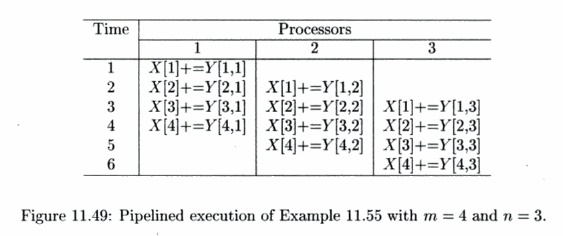
Successive  over-relaxation  (SOR) is  a  technique  for  accelerating  the  convergence of relaxation methods for solving sets of simultaneous linear equations.

A relatively simple template illustrating its data-access pattern is shown in Fig. 11.50(a). Here, the new value of an element in the array depends on the values of elements in its neighborhood. Such an operation is performed repeat-edly, until some convergence criterion is met.

Shown in Fig. 11.50(b) is a picture of the key data dependences. We do not show dependences that can be inferred by the dependences already included in the figure. For example, iteration [i,j] depends on iterations [i,j — 1], [i,j — 2] and so on. It is clear from the dependences that there is no synchronization-free parallelism. Since the longest chain of dependences consists of 0(m + n) edges, by introducing synchronization, we should be able to find one degree of parallelism and execute the 0(mn) operations in 0(m + n) unit time.

In particular, we observe that iterations that lie along the 150° diagonals7 in Fig. 11.50(b) do not share any dependences. They Only depend on the iterations that lie along diagonals closer to the origin. Therefore we can parallelize this code by executing iterations on each diagonal in order, starting at the origin and proceeding outwards. We refer to the iterations along each diagonal as a wavefront, and such a parallelization scheme as wavefronting.

3. Fully Permutable Loops

We first introduce the notion of full permutability, a concept useful for pipelining and other optimizations. Loops are fully permutable if they can be permuted arbitrarily without changing the semantics of the original program. Once loops are put in a fully permutable form, we can easily pipeline the code and apply transformations such as blocking to improve data locality.

The SOR code, as it it written in Fig. 11.50(a), is not fully permutable. As shown in Section 11.7.8, permuting two loops means that iterations in the original iteration space are executed column by column instead of row by row. For instance, the original computation in iteration [2,3] would execute before that of [1,4], violating the dependences shown in Fig. 11.50(b).

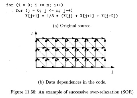
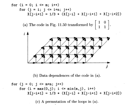
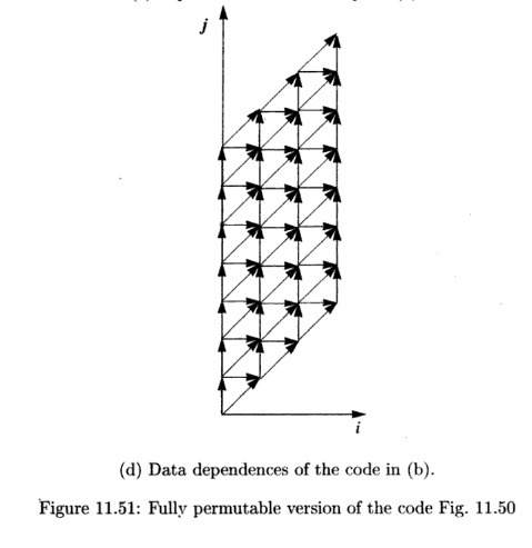
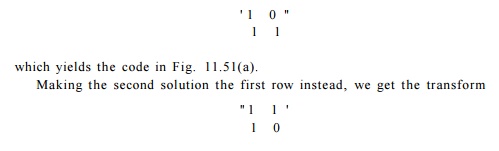
We can, however, transform the code to make it fully permutable. Applying the affine transform

to the code yields the code shown in Fig. 11.51(a). This transformed code is fully permutable, and its permuted version is shown in Fig. 11.51(c). We also show the iteration space and data dependences of these two programs in Fig. 11.51(b) and (d), respectively. From the figure, we can easily see that this ordering preserves the relative ordering between every data-dependent pair of accesses.

When we permute loops, we change the set of operations executed in each iteration of the outermost loop drastically.    The fact that we have this degree of freedom  in  scheduling means  that  there       is  a lot  of slack in  the  ordering of operations in the program. Slack in scheduling means opportunities for parallelization. We show later in this section that if a loop has k outermost fully permutable loops, by introducing just 0(n)  synchronizations, we can get 0(k - 1)  degrees of parallelism (n is the number of iterations in a loop).

4. Pipelining Fully Permutable Loops

A loop with k outermost fully permutable loops can be structured as a pipeline with 0(k - 1) dimensions. In the SOR example, k = 2, so we can structure the processors as a linear pipeline.

We can pipeline the SOR code in two different ways, shown in Fig. 11.52(a) and Fig. 11.52(b), corresponding to the two possible permutations shown in Fig. 11.51(a) and (c), respectively. In each case, every column of the iteration space constitutes a task, and every row constitutes a stage. We assign stage i to processor i, thus each processor executes the inner loop of the code. Ignoring boundary conditions, a processor can execute iteration i only after processor p — 1 has executed iteration i — 1.

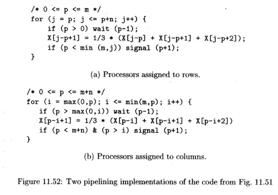
Suppose every processor takes exactly the same amount of time to execute an iteration and synchronization happens instantaneously. Both these pipelined schemes would execute the same iterations in parallel; the only difference is that they have different processor assignments. All the iterations executed in parallel lie along the 135° diagonals in the iteration space in Fig. 11.51(b), which corresponds to the 150° diagonals in the iteration space of the original code; see Fig. 11.50(b).

However, in practice, processors with caches do not always execute the same code in the same amount of time, and the time for synchronization also varies. Unlike the use of synchronization barriers which forces all processors to operate in lockstep, pipelining requires processors to synchronize and communicate with at most two other processors. Thus, pipelining has relaxed wavefronts, allowing some processors to surge ahead while others lag momentarily. This flexibility reduces the time processors spend waiting for other processors and improves parallel performance.

The two pipelining schemes  shown  above are but  two of the many ways in which the computation can be pipelined.  As we said, once a loop is fully permutable, we have a lot of freedom in how we wish to parallelize the code.

The first pipeline scheme maps iteration to processor i; the second maps iteration to processor j.  We can create alternative pipelines by mapping iteration to processor CQI + cij, provided CQ and c1 are positive constants.

Such a scheme would create pipelines with relaxed wavefronts between 90° and 180°, both exclusive.

5. General Theory

The example just completed illustrates the following general theory underlying pipelining: if we can come up with at least two different outermost loops for a loop nest and satisfy all the dependences, then we can pipeline the computation. A loop with k outermost fully permutable loops has k — 1 degrees of pipelined parallelism.

Loops that cannot be pipelined do not have alternative outermost loops. Example 11.56 shows one such instance. To honor all the dependences, each iteration in the outermost loop must execute precisely the computation found in the original code. However, such code may still contain parallelism in the inner loops, which can be exploited by introducing at least n synchronizations, where n is the number of iterations in the outermost loop.

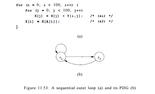
Example 11. 56 : Figure 11.53 is a more complex version of the problem we saw in Example 11.50. As shown in the program dependence graph in Fig. 11.53(b), statements s1 and s2 belong to the same strongly connected component. Be-cause we do not know the contents of matrix A, we must assume that the access in statement s2 may read from any of the elements of X. There is a true dependence from statement si to statement s2 and an antidependence from statement s2 to statement s x . There is no opportunity for pipelining either, because all operations belonging to iteration i in the outer loop must precede those in iteration i + To find more parallelism, we repeat the parallelization process on the inner loop. The iterations in the second loop can be parallelized without synchronization. Thus, 200 barriers are needed, with one before and one after each execution of the inner loop. •

6. Time-Partition Constraints

We now focus on the problem of finding pipelined parallelism. Our goal is to turn a computation into a set of pipelinable tasks. To find pipelined parallelism, we do not solve directly for what is to be executed on each processor, like we did with loop parallelization. Instead, we ask the following fundamental ques-tion: What are all the possible execution sequences that honor the original data dependences in the loop? Obviously the original execution sequence satisfies all the data dependences. The question is if there are affine transformations that can create an alternative schedule, where iterations of the outermost loop exe-cute a different set of operations from the original, and yet all the dependences are satisfied. If we can find such transforms, we can pipeline the loop. The key point is that if there is freedom in scheduling operations, there is paral-lelism; details of how we derive pipelined parallelism from such transforms will be explained later.

To find acceptable reorderings of the outer loop, we wish to find one-dimensional affine transforms, one for each statement, that map the original loop index values to an iteration number in the outermost loop. The trans-forms are legal if the assignment can satisfy all the data dependences in the program. The "time-partition constraints," shown below, simply say that if one operation is dependent upon the other, then the first must be assigned an iteration in the outermost loop no earlier than that of the second. If they are assigned in the same iteration, then it is understood that the first will be executed after than the second within the iteration.

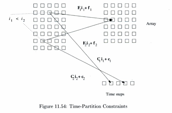
An affine-partition mapping of a program is a legal-time partition if and only if for every two (not necessarily distinct) accesses sharing a dependence, say

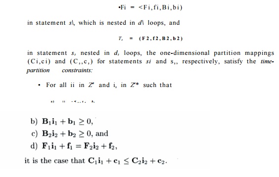
This constraint, illustrated in Fig. 11.54, looks remarkably similar to the space-partition constraints. It is a relaxation of the space-partition constraints, in that if two iterations refer to the same location, they do not necessarily have to be mapped to the same partition; we only require that the original relative execution order between the two iterations is preserved. That is, the constraints here have < where the space-partition constraints have =.

We know that there exists at least one solution to the time-partition con-straints. We can map operations in each iteration of the outermost loop back to the same iteration, and all the data dependences will be satisfied. This so-lution is the only solution to the time-partition constraints for programs that cannot be pipelined. On the other hand, if we can find several independent solutions to time-partition constraints, the program can be pipelined. Each independent solution corresponds to a loop in the outermost fully permutable nest. As you can expect, there is only one independent solution to the timing constraints extracted from the program in Example 11.56, where there is no pipelined parallelism, and that there are two independent solutions to the SOR code example.

Example 1 1 . 5 7 : Let us consider Example 11.56, and in particular the data dependences of references to array X in statements si and s 2 . Because the access is not affine in statement s2, we approximate the access by modeling matrix X simply as a scalar variable in dependence analysis involving statement s2. Let be the index value of a dynamic instance of si and let %' be the index value of a dynamic instance of s2. Let the computation mappings of statements s1, and s2 be ([Cn,C12],c1) and ([C2i],C2), respectively.

Similar arguments about the data dependence from s2 to si and s2 back to itself will yield a similar answer. In this particular solution, the zth iteration of the outer loop, which consists of the instance i of s2 and all instances of si, are all assigned to timestep i. Other legal choices of Cn, C2i, ci, and C2 yield similar assignments, although there might be timesteps at which nothing happens. That is, all ways to schedule the outer loop require the iterations to execute in the same order as in the original code. This statement holds whether all 100 iterations are executed on the same processor, on 100 different processors, or anything in between. •

Example 1 1 . 5 8 :  In the SOR code shown in Fig. 11.50(a), the write reference X[j + 1]  shares a dependence with itself and with the three read references in the code. We are seeking computation mapping ([C±, C2], c) for the assignment statement such that

1.  True dependence from write access X[j +1 ] to read access X[j + 2]. Since the instances must access the same location, j + 1 = j' + 2 or j = j' + 1.

Substituting j = j' + 1 into the timing constraints, we get 

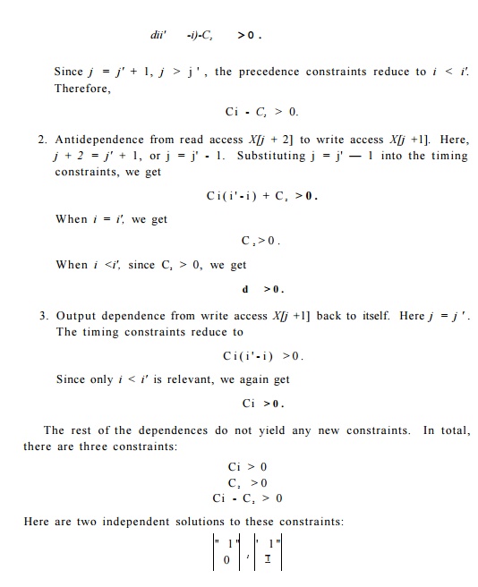
The first solution preserves the execution order of the iterations in the outer-most loop. Both the original SOR code in Fig. 11.50(a) and the transformed code shown in Fig. 11.51(a) are examples of such an arrangement. The second solution places iterations lying along the 135° diagonals in the same outer loop. The code shown in Fig. 11.51(b) is an example of a code with that outermost loop composition.

Notice that there are many other possible pairs of independent  solutions.

For example,

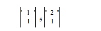
would also be an independent solutions to the same constraints. We choose the simplest vectors to simplify code transformation.

7. Solving Time-Partition Constraints by Farkas' Lemma

Since time-partition constraints are similar to space-partition constraints, can we use a similar algorithm to solve them? Unfortunately, the slight difference between the two problems translates into a big technical difference between the two solution methods. Algorithm 11.43 simply solves for C 1 , c 1 , C 2 , and c 2 , such that for all ii in Zdl  and i2 in Zd2 if

The linear inequalities due to the loop bounds are only used in determining if two references share a data dependence, and are not used otherwise.

To find solutions to the time-partition constraints, we cannot ignore the linear inequalities i -< i'; ignoring them often would allow only the trivial so-lution of placing all iterations in the same partition. Thus, the algorithm to find solutions to the time-partition constraints must handle both equalities and inequalities linear inequalities i -< i'; ignoring them often would allow only the trivial solution of placing all iterations in the same partition. Thus, the algorithm to find solutions to the time-partition constraints must handle both equalities and  inequalities.

The general problem we wish to solve is: given a matrix A, find a vector c such that for all vectors x such that Ax > 0, it is the case that c T x >  0.

In other words, we are seeking c such that the inner product of c and any coordinates in the polyhedron defined by the inequalities Ax > 0 always yields a nonnegative answer.

This problem is addressed by Farkas' Lemma. Let A be an m x n matrix of reals, and let c be a real, nonzero n-vector. Farkas' lemma says that either the primal system of inequalities

A x > 0,                         c T x < 0

 has a real-valued solution x, or the dual system

A T  y = c,                        y > 0

 has a real-valued solution y, but never both.

The dual system can be handled by using Fourier-Motzkin elimination to project away the variables of y. For each c that has a solution in the dual system, the lemma guarantees that there are no solutions to the primal system. Put another way, we can prove the negation of the primal system, i.e., we can  prove that c T x >    0 for  all x such that Ax > 0, by finding a solution y to the dual system:  A T y = c and y > 0.

Algorithm 11.59 : Finding a set of legal, maximally independent affine time-partition mappings for an outer sequential loop.

About Farkas' Lemma

The proof of the lemma can be found in many standard texts on linear programming. Farkas' Lemma, originally proved in 1901, is one of the theorems of the alternative. These theorems are all equivalent but, despite attempts over the years, a simple, intuitive proof for this lemma or any of its equivalents has not been found.

INPUT: A loop nest with array accesses.

OUTPUT: A maximal set of linearly independent time-partition mappings.

METHOD: The following steps constitute the algorithm:

1. Find all data-dependent pairs of accesses in a program.

2. For each pair of data-dependent accesses, T1 = ( F i , f i , B i , b i ) in statement si nested in d1 loops and T2 — ( F 2 , f2, B 2 , b 2 ) in statement s2 nested in d2 loops, let (Ci ,Ci) and ( C 2 , c 2 ) be the (unknown) time-partition mappings of statements si and s 2 , respectively. Recall the time-partition constraints state that

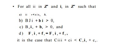
Since ii -<gl S 2 h is a disjunctive union of a number of clauses, we can create a system of constraints for each clause and solve each of them separately, as follows:

(a) Similarly to step (2a) in Algorithm 11.43, apply Gaussian elimination to the equations

(b)                     Let c be all the unknowns in the partition mappings. Express the linear inequality constraints due to the partition mappings as

c T D x  >= 0

for some matrix D.

(c)                     Express the precedence constraints on the loop index variables and the loop bounds as

A x > =0

for some matrix A.

(d)                    Apply Farkas'Lemma. Finding x to satisfy the two constraints above is equivalent to finding y such that

A T  y = D T  c and y >= 0.

Note that c T D here is cT in the statement of Farkas' Lemma, and we are using the negated form of the lemma.

(e)                     In this form, apply Fourier-Motzkin elimination to project away the y variables, and express the constraints on the coefficients c as Ec >= 0.

(f)                      Let E'c' > = 0 be the system without the constant terms.

3.         Find a maximal set of linearly independent solutions to E'c'  > =0 using Algorithm B.I in Appendix B. The approach of that complex algorithm is to keep track of the current set of solutions for each of the statements, then incrementally look for more independent solutions by inserting con-straints that force the solution to be linearly independent for at least one statement.

4.         From each solution of c' found, derive one affine time-partition mapping. The constant terms are derived using Ec > = 0.

Example 11 . 60: The constraints for Example 11.57 can be written as

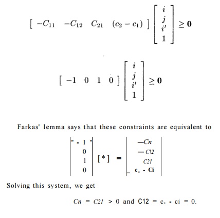
Notice that these constraints are satisfied by the particular solution we obtained in Example 11.57. •

8. Code Transformations

If there exist k independent solutions to the time-partition constraints of a loop nest, then it is possible to transform the loop nest to have k outermost fully permutable loops, which can be transformed to create k—1 degrees of pipelining, or to create k — 1 inner parallelizable loops. Furthermore, we can apply blocking to fully permutable loops to improve data locality of uniprocessors as well as reducing synchronization among processors in a parallel execution.

E x p l o i t i n g  Fully  P e r m u t a b l e  L o o p s

We can create a loop nest with k outermost fully permutable loops easily from

k independent solutions to the time-partition constraints. We can do so by simply making the kth. solution the kih row of the new transform. Once the affine transform is created, Algorithm 11.45 can be used to generate the code.

Example 1 1 . 6 1 : The solutions found in Example 11.58 for our SOR example were

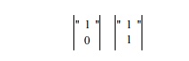
Making the first solution the first row and the second solution the second row, we get the transform

It is easy to see that such transforms produce a legal sequential program. The first row partitions the entire iteration space according to the first solution. The timing constraints guarantee that such a decomposition does not violate any data dependences. Then, we partition the iterations in each of the outer-most loop according to the second solution. Again this must be legal because we are dealing with just subsets of the original iteration space. The same goes for the rest of the rows in the matrix. Since we can order the solutions arbitrarily, the loops are fully permutable.

Exploiting  Pipelining

We can easily transform a loop with k outermost fully permutable loops into a code with k — 1 degrees of pipeline parallelism.

Exampl e 1 1 . 6 2 : Let us return to our SOR example. After the loops are transformed to be fully permutable, we know that iteration [k, i2] can be exe-cuted provided iterations [k,k — 1] and [k — 1,^] have been executed. We can guarantee this order in a pipeline as follows. We assign iteration k to processor pi. Each processor executes iterations in the inner loop in the original sequen-tial order, thus guaranteeing that iteration [k,i2] executes after [ii,i2 — 1]. In addition, we require that processor p waits for the signal from processor p — 1 that it has executed iteration [p — l,i2] before it executes iteration [p,«V|. This technique generates the pipelined code Fig. 11.52(a) and (b) from the fully permutable loops Fig. 11.51(a) and (c), respectively. •

In general, given k outermost fully permutable loops, the iteration with index values (ii,... ,ik) can be executed without violating data-dependence constraints, provided iterations

have been executed. We can thus assign the partitions of the first k — 1 dimen-sions of the iteration space to 0 ( n f e _ 1 ) processors as follows. Each processor is responsible for one set of iterations whose indexes agree in the first k — 1 dimen-sions, and vary over all values of the kth index. Each processor executes the iterations in the kth loop sequentially. The processor corresponding to values [pi,p 2 , • • • ,Pk-i] for the first k — 1 loop indexes can execute iteration i in the feth loop as long as it receives a signal from processors

that they have executed their ith iteration in the kth loop.

Wavefr ont ing

It is also easy to generate k — 1 inner parallelizable loops from a loop with k outermost fully permutable loops. Although pipelining is preferable, we include this information here for completeness.

We partition the computation of a loop with k outermost fully permutable loops using a new index variable i': where i' is defined to be some combination of all the indices in the k permutable loop nest. For example, i' = i± + ... + ik is one such combination.

We create an outermost sequential loop that iterates through the i' par-titions in increasing order; the computation nested within each partition is ordered as before. The first k - 1 loops within each partition are guaranteed to be parallelizable. Intuitively, if given a two-dimensional iteration space, this transform groups iterations along 135° diagonals as an execution of the outer-most loop. This strategy guarantees that iterations within each iteration of the outermost loop have no data dependence.

Blocking

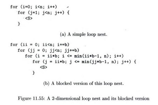
A k-deep, fully permutable loop nest can be blocked in ^-dimensions. Instead of assigning the iterations to processors based on the value of the outer or inner loop indexes, we can aggregate blocks of iterations into one unit. Blocking is useful for enhancing data locality as well as for minimizing the overhead of pipelining.

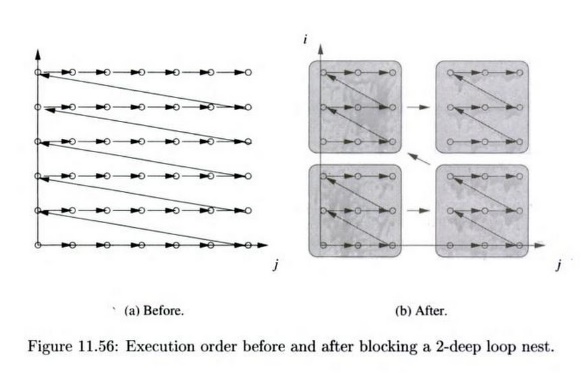
Suppose we have a two-dimensional fully permutable loop nest, as in Fig. 11.55(a), and we wish to break the computation into b x b blocks. The execution order of the blocked code is shown in Fig. 11.56, and the equivalent code is in Fig. 11.55(b).

If we assign each block to one processor, then all the passing of data from one iteration to another that is within a block requires no interprocessor communi-cation. Alternatively, we can coarsen the granularity of pipelining by assigning a column of blocks to one processor. Notice that each processor synchronizes with its predecessors and successors only at block boundaries. Thus, another advantage of blocking is that programs only need to communicate data ac-cessed at the boundaries of the block with their neighbor blocks. Values that are interior to a block are managed by only one processor.

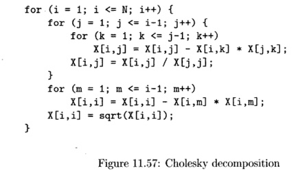
Example 1 1 . 6 3 : We now use a real numerical algorithm — Cholesky decom-position — to illustrate how Algorithm 11.59 handles single loop nests with only pipelining parallelism. The code, shown in Fig. 11.57, implements an 0 ( n 3 ) al-gorithm, operating on a 2-dimensional data array. The executed iteration space is a triangular pyramid, since j only iterates up to the value of the outer loop index i, and k only iterates to the value of j. The loop has four statements, all nested in different loops.

Applying Algorithm 11.59 to this program finds three legitimate time di-mensions. It nests all the operations, some of which were originally nested in 1- and 2-deep loop nests into a 3-dimensional, fully permutable loop nest. The code, together with the mappings, is shown in Fig. 11.58.

The code-generation routine guards the execution of the operations with the original loop bounds to ensure that the new programs execute only operations

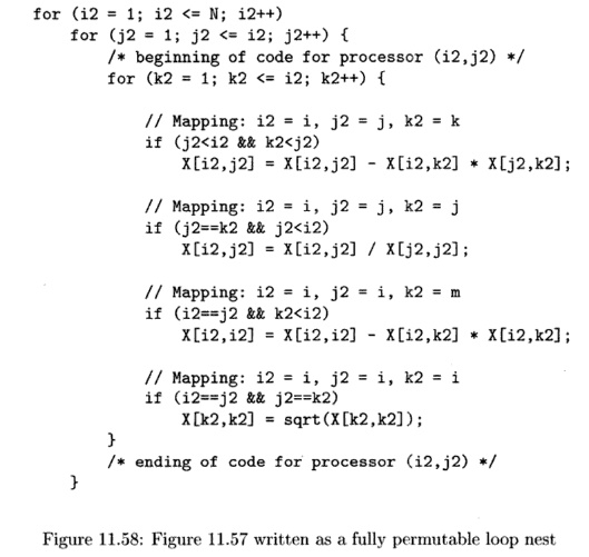
that are in the original code. We can pipeline this code by mapping the 3-dimensional structure to a 2-dimensional processor space. Iterations (i2,j2, k2) are assigned to the processor with ID (i2,j2). Each processor executes the innermost loop, the loop with the index k2. Before it executes the kth iteration, the processor waits for signals from the processors with ID's (%2 — l,j2) and (i2,j2 - 1). After it executes its iteration, it signals processors (12 + l , j 2 ) and (*2,j2 + l) . •

9. Parallelism With Minimum Synchronization

We have described three powerful parallelization algorithms in the last three sections: Algorithm 11.43 finds all parallelism requiring no synchronizations, Algorithm 11.54 finds all parallelism requiring only a constant number of syn-chronizations, and Algorithm 11.59 finds all the pipelinable parallelism requir-ing 0(n) synchronizations where n is the number of iterations in the outermost loop. As a first approximation, our goal is to parallelize as much of the compu-tation as possible, while introducing as little synchronization as necessary.

Algorithm 11.64, below, finds all the degrees of parallelism in a program, starting with the coarsest granularity of parallelism. In practice, to parallelize a code for a multiprocessor, we do not need to exploit all the levels of parallelism, just the outermost possible ones until all the computation is parallelized and all the processors are fully utilized.

Algorithm 11.64 : Find all the degrees of parallelism in a program, with all the parallelism being as coarse-grained as possible.

INPUT: A program to be parallelized.

OUTPUT: A parallelized version of the same program.

METHOD: Do the following:

1.         Find the maximum degree of parallelism requiring no synchronization: Apply Algorithm 11.43 to the program.

2.          Find the maximum degree of parallelism that requires 0(1) synchroniza-tions: Apply Algorithm 11.54 to each of the space partitions found in step 1. (If no synchronization-free parallelism is found, the whole compu-tation is left in one partition).

3.         Find the maximum degree of parallelism that requires 0(n)  synchroniza-

tions. Apply Algorithm 11.59 to each of the partitions found in step 2 to find pipelined parallelism. Then apply Algorithm 11.54 to each of the partitions assigned to each processor, or the body of the sequential loop if no pipelining is found.

4. Find the maximum degree of parallelism with successively greater degrees of synchronizations: Recursively apply Step 3 to computation belonging to each of the space partitions generated by the previous step.

Example 11.65 : Let us now return to Example 11.56. No parallelism is found by Steps 1 and 2 of Algorithm 11.54; that is, we need more than a constant number of synchronizations to parallelize this code. In Step 3, applying Algorithm 11.59 determines that there is only one legal outer loop, which is the one in the original code of Fig. 11.53. So, the loop has no pipelined parallelism. In the second part of Step 3, we apply Algorithm 11.54 to parallelize the inner loop. We treat the code within a partition like a whole program, the only difference being that the partition number is treated like a symbolic constant. In this case the inner loop is found to be parallelizable and therefore the code can be parallelized with n synchronization barriers. •

Algorithm 11.64 finds all the parallelism in a program at each level of syn-chronization. The algorithm prefers parallelization schemes that have less syn-chronization, but less synchronization does not mean that the communication is minimized. Here we discuss two extensions to the algorithm to address its weaknesses.

Considering  Communication  Cost

Step 2 of Algorithm 11.64 parallelizes each strongly connected component in-dependently if no synchronization-free parallelism is found. However, it may be possible to parallelize a number of the components without synchronization and communication. One solution is to greedily find synchronization-free par-allelism among subsets of the program dependence graph that share the most data.

If communication is necessary between strongly connected components, we note that some communication is more expensive than others. For example, the cost of transposing a matrix is significantly higher than just having to com-municate between neighboring processors. Suppose si and s2 are statements in two separate strongly connected components accessing the same data in iterations ii and i 2 , respectively. If we cannot find partition mappings ( C i , c i ) and ( C 2 , c 2 ) for statements si and s 2 , respectively, such that

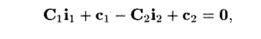
we instead try to satisfy the constraint

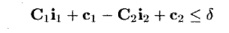
where S is a small constant.

Trading  Communication for  Synchronization

Sometimes we would rather perform more synchronizations to minimize com-munication. Example 11.66 discusses one such example. Thus, if we cannot parallelize a code with just neighborhood communication among strongly con-nected components, we should attempt to pipeline the computation instead of parallelizing each component independently. As shown in Example 11.66, pipelining can be applied to a sequence of loops.

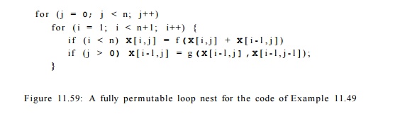
E x a m p l e 11 . 66: For the ADI integration algorithm in Example 11.49, we have shown that optimizing the first and second loop nests independently finds parallelism in each of the nests. However, such a scheme would require that the matrix be transposed between the loops, incurring 0 ( n 2 ) data traffic. If we use Algorithm 11.59 to find pipelined parallelism, we find that we can turn the entire program into a fully permutable loop nest, as in Fig. 11.59. We then can apply blocking to reduce the communication overhead. This scheme would incur 0(n) synchronizations but would require much less communication.

10. Exercises for Section 11.9

Exercise 1 1 . 9 , 1 : In Section 11.9.4, we discussed the possibility of using diagonals other than the horizontal and vertical axes to pipeline the code of Fig. 11.51.  Write code analogous to the loops of Fig. 11.52 for the diagonals:

(a) 135° (b) 120°.

Exercise 11 . 9 . 2: Figure 11.55(b) can be simplified if b divides n evenly. Rewrite the code under that assumption.

for (i=0; i<100; i++) { P[i,0] = 1; /* si */ P[i,i] = 1; /* s2 */

}

for (i=2; i<100; i++) for (j=l; j<i; j++)

P[i,j]  = P[i-l,j-l]  + P[i-l,j];   /*  s3 */

Figure 11.60:  Computing Pascal's triangle

Exercise 1 1 . 9 . 3 : In Fig. 11.60 is a program to compute the first 100 rows of Pascal's triangle. That is, P[i,j] will become the number of ways to choose j things out of i, for 0 < j < i < 100.

a)             Rewrite the code as a single, fully permutable loop nest.

b)        Use 100 processors in a pipeline to implement this code.  Write the code for each processor p, in terms of p, and indicate the synchronization necessary.

c) Rewrite the code using square blocks of 10 iterations on a side. Since the iterations form a triangle, there will be only 1 + 2-1 h 10 = 55 blocks.

Show the code for a processor ( p i ,P2) assigned to the pith block in the i direction and the p 2 t h block in the j direction, in terms of pi and p2.

Exercise 1 1 . 9 . 4 : Repeat Exercise 11.9.2 for the code of Fig. 11.61. However, note that the iterations for this problem form a 3-dimensional cube of side 100. Thus, the blocks for part (c) should be 10 x 10 x 10, and there are 1000 of them.

 Exercise 1 1 . 9 . 5 : Let us apply Algorithm 11.59 to a simple example of the time-partition constraints. In what follows, assume that the vector ii is and vector i2 is (i2,j2); technically, both these vectors are transposed. The condition ii -<Sls2 *2 consists of the following disjunction:

The other equalities and inequalities are

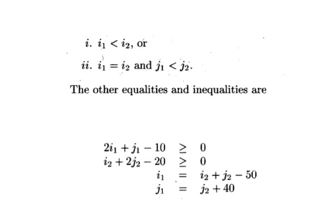
Finally, the time-partition inequality, with unknowns c1, d1, e1, c2, d2, and e 2 , is

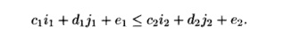
a) Solve the time-partition constraints for case i — that is, where i1 < i 2 . In particular, eliminate as many of i1, j±, i2, and j2 as you can, and set up the matrices D and A as in Algorithm 11.59. Then, apply Farkas' Lemma to the resulting matrix inequalities.

b) Repeat part (a) for the case ii, where i1 — i2 and ji < j 2 .