Matrix Multiply: An In-Depth Example

Matrix Multiply: An In-Depth Example

1 The Matrix-Multiplication Algorithm

2 Optimizations

3 Cache Interference

4 Exercises for Section 11.2

We shall introduce many of the techniques used by parallel compilers in an ex-tended example. In this section, we explore the familiar matrix-multiplication algorithm to show that it is nontrivial to optimize even a simple and easily parallelizable program. We shall see how rewriting the code can improve data locality; that is, processors are able to do their work with far less communica-tion (with global memory or with other processors, depending on the architec-ture) than if the straightforward program is chosen. We shall also discuss how cognizance of the existence of cache lines that hold several consecutive data ele-ments can improve the running time of programs such as matrix multiplication.

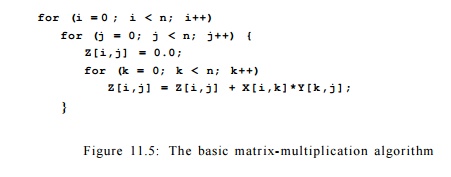
1. The Matrix-Multiplication Algorithm

In Fig. 11.5 we see a typical matrix-multiplication program.² It takes two nxn matrices, X and F, and produces their product in a third n x n matrix Z. Recall that % — the element of matrix Z in row i and column j — must become YJl=i  ^-ihXkj-

The code of Fig. 11.5 generates n² results, each of which is an inner product between one row and one column of the two matrix operands. Clearly, the ² In pseudocode programs in this chapter, we shall generally use C syntax, but to make multidimensional array accesses — the central issue for most of the chapter — easier to read, we shall use Fortran-style array references, that is, Z[i,j] instead of

calculations of each of the elements of Z are independent and can be executed in parallel.

The larger n is, the more times the algorithm touches each element. That is, there are 3 n 2 locations among the three matrices, but the algorithm performs n3 operations, each of which multiplies an element of X by an element of Y and adds the product to an element of Z. Thus, the algorithm is computation-intensive and memory accesses should not, in principle, constitute a bottleneck.

Serial Execution of the  Matrix  Multiplication

Let us first consider how this program behaves when run sequentially on a uniprocessor. The innermost loop reads and writes the same element of Z, and uses a row of X and a column of Y. Z[i,j] can easily be stored in a register and requires no memory accesses. Assume, without loss of generality, that the matrix is laid out in row-major order, and that c is the number of array elements in a cache line.

Figure 11.6 suggests the access pattern as we execute one iteration of the outer loop of Fig. 11.5. In particular, the picture shows the first iteration, with i = 0. Each time we move from one element of the first row of X to the next, we visit each element in a single column of Y. We see in Fig. 11.6 the assumed organization of the matrices into cache lines. That is, each small rectangle represents a cache line holding four array elements (i.e., c = 4 and n = 12 in the picture).

Accessing X puts little burden on the cache. One row of X is spread among only n/c cache lines. Assuming these all fit in the cache, only n/c cache misses occur for a fixed value of index i, and the total number of misses for all of X is n²/c, the minimum possible (we assume n is divisible by c, for convenience).

However, while using one row of X, the matrix-multiplication algorithm accesses all the elements of Y, column by column. That is, when j = 0, the inner loop brings to the cache the entire first column of Y. Notice that the elements of that column are stored among n different cache lines. If the cache is big enough (or n small enough) to hold n cache lines, and no other uses of the cache force some of these cache lines to be expelled, then the column for j = 0 will still be in the cache when we need the second column of Y. In that case, there will not be another n cache misses reading Y, until j = c, at which time we need to bring into the cache an entirely different set of cache lines for Y. Thus, to complete the first iteration of the outer loop (with i = 0) requires between n 2 / c and n2 cache misses, depending on whether columns of cache lines can survive from one iteration of the second loop to the next.

Moreover, as we complete the outer loop, for i = 1,2, and so on, we may have many additional cache misses as we read Y, or none at all. If the cache is big enough that all n 2 / c cache lines holding Y can reside together in the cache, then we need no more cache misses. The total number of cache misses is thus 2 n 2 / c , half for X and half for Y. However, if the cache can hold one column of Y but not all of Y, then we need to bring all of Y into cache again, each time we perform an iteration of the outer loop. That is, the number of cache misses is n 2 / c + n 3 / c ; the first term is for X and the second is for Y. Worst, if we cannot even hold one column of Y in the cache, then we have n2 cache misses per iteration of the outer loop and a total of n 2 / c + n3 cache misses.

Row - by - Row Parallelization

Now, let us consider how we could use some number of processors, say p proces-sors, to speed up the execution of Fig. 11.5. An obvious approach to parallelizing matrix multiplication is to assign different rows of Z to different processors. A processor is responsible for n/p consecutive rows (we assume n is divisible by p, for convenience). With this division of labor, each processor needs to access n/p rows of matrices X and Z, but the entire Y matrix. One processor will compute n² jp elements of Z, performing n³/p multiply-and-add operations to do so.

While the computation time thus decreases in proportion to p, the communication cost  actually rises in proportion to p.  That is,  each of p processors has to read n2/p elements of X,  but all n2    elements of Y.  The total number of cache lines that must be delivered to the caches of the p processors is at last n 2 / c + p n 2 / c ; the two terms are for delivering X and copies of Y, respectively.

As p approaches n, the computation time becomes 0 ( n 2 ) while the communi-cation cost is 0 ( n 3 ) . That is, the bus on which data is moved between memory and the processors' caches becomes the bottleneck. Thus, with the proposed data layout, using a large number of processors to share the computation can actually slow down the computation, rather than speed it up.

2. Optimizations

The matrix-multiplication algorithm of Fig.  11.5 shows that even though an algorithm may reuse the same data, it may have poor data locality.  A reuse of data results in a cache hit only if the reuse happens soon enough, before the data is displaced from the cache. In this case, n² multiply-add operations separate the reuse of the same data element in matrix Y, so locality is poor. In fact, n operations separate the reuse of the same cache line in Y. In addi-tion, on a multiprocessor, reuse may result in a cache hit only if the data is reused by the same processor. When we considered a parallel implementation in Section 11.2.1, we saw that elements of Y had to be used by every processor. Thus, the reuse of Y is not turned into locality.

Changing  D a t a  Layout

One way to improve the locality of a program is to change the layout of its data structures. For example, storing Y in column-major order would have improved the reuse of cache lines for matrix Y. The applicability of this approach is limited, because the same matrix normally is used in different operations. If Y played the role of X in another matrix multiplication, then it would suffer from being stored in column-major order, since the first matrix in a multiplication is better stored in row-major order.

Blocking

It is sometimes possible to change the execution order of the instructions to improve data locality. The technique of interchanging loops, however, does not improve the matrix-multiplication routine. Suppose the routine were written to generate a column of matrix Z at a time, instead of a row at a time. That is, make the j - loop the outer loop and the z-loop the second loop. Assuming matrices are still stored in row-major order, matrix Y enjoys better spatial and temporal locality, but only at the expense of matrix X.

Blocking is another way of reordering iterations in a loop that can greatly improve the locality of a program. Instead of computing the result a row or a column at a time, we divide the matrix up into submatrices, or blocks, as suggested by Fig. 11.7, and we order operations so an entire block is used over a short period of time. Typically, the blocks are squares with a side of length  B. If B evenly divides n, then all the blocks are square. If B does not evenly divide n, then the blocks on the lower and right edges will have one or both sides of length less than B.

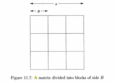
Figure 11.8 shows a version of the basic matrix-multiplication algorithm where all three matrices have been blocked into squares of side B. As in Fig. 11.5, Z is assumed to have been initialized to all O's. We assume that B divides n; if not, then we need to modify line (4) so the upper limit is min(u + B,n), and similarly for lines (5) and (6).

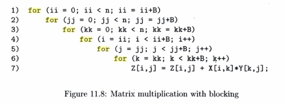
The outer three loops, lines (1) through (3), use indexes ii,     jj, and kk,   which are always incremented by B, and therefore always mark the left or upper edge of some blocks. With fixed values of ii, jj, and kk, lines (4) through (7) enable the blocks with upper-left corners X[ii,kk] and Y[kk,jj] to make all possible contributions to the block with upper-left corner Z[ii,jj).

If we pick B properly, we can significantly decrease the number of cache misses, compared with the basic algorithm, when all of X, Y, or Z cannot fit in the cache. Choose B such that it is possible to fit one block from each of the matrices in the cache. Because of the order of the loops, we actually need each block of Z in cache only once, so (as in the analysis of the basic algorithm in Section 11.2.1) we shall not count the cache misses due to Z.

Another View of Block-Based Matrix Multiplication

We can imagine that the matrices X,Y, and Z of Fig.  11.8 are not n x n matrices  of  floating-point  numbers,  but  rather (n/B)  x  (n/B) matrices whose elements are themselves B x B matrices of floating-point numbers.  Lines (1) through (3) of Fig. 11.8 are then like the three loops of the basic algorithm in Fig. 11.5, but with n/B as the size of the matrices, rather than n. We can then think of lines (4) through (7) of Fig. 11.8 as implementing a single multiply-and-add operation of Fig. 11.5. Notice that in this operation, the single multiply step is a matrix-multiply step, and it uses the basic algorithm of Fig. 11.5 on the floating-point numbers that are elements of the two matrices involved. The matrix addition is element-wise addition of floating-point numbers.

To bring a block of X or Y to the cache takes B²/c cache misses; recall c is the number of elements in a cache line. However, with fixed blocks from X and Y, we perform B³ multiply-and-add operations in lines (4) through (7) of Fig. 11.8. Since the entire matrix-multiplication requires n³ multiply-and-add operations, the number of times we need to bring a pair of blocks to the cache

is n ³ / B ³ .  As we require 2B²/c cache misses each time we do, the total number of cache  misses  is  2n³/Bc.

It is interesting to compare this figure 2n3/Be with the estimates given in Section 11.2.1. There, we said that if entire matrices can fit in the cache, then 0 ( n 2 / c ) cache misses suffice.  However, in that case, we can pick B = n, i.e., make each matrix be a single block.  We again get 0 ( n 2 / c ) as our estimate of cache misses.  On the other hand, we observed that if entire matrices will not fit in cache, we require 0 ( n 3 / c ) cache misses, or even 0 ( n 3 ) cache misses. In that case, assuming that we can still pick a significantly large B  (e.g., B could be 200, and we could still fit three blocks of 8-byte numbers in a one-megabyte cache), there is a great advantage to using blocking in matrix multiplication.

The blocking technique can be reapplied for each level of the memory hi-erarchy. For example, we may wish to optimize register usage by holding the operands of a 2 x 2 matrix multiplication in registers. We choose successively bigger block sizes for the different levels of caches and physical memory.

Similarly, we can distribute blocks between processors to minimize data traf-fic. Experiments showed that such optimizations can improve the performance of a uniprocessor by a factor of 3, and the speed up on a multiprocessor is close to linear with respect to the number of processors used.

3. Cache Interference

Unfortunately, there is somewhat more to the story of cache utilization.  Most caches are not fully associative (see Section 7.4.2).  In a direct-mapped cache, if n is a multiple of the cache size, then all the elements in the same row of an n x n array will be competing for the same cache location. In that case, bringing in the second element of a column will throw away the cache line of the first, even though the cache has the capacity to keep both of these lines at the same time.  This situation is referred to as  cache  interference.

There are various solutions to this problem. The first is to rearrange the data once and for all so that the data accessed is laid out in consecutive data locations. The second is to embed the n x n array in a larger mxn array where m is chosen to minimize the interference problem. Third, in some cases we can choose a block size that is guaranteed to avoid interference.

4. Exercises for Section 11.2

Exercise 1 1 . 2 . 1 :  The block-based  matrix-multiplication  algorithm  of Fig. 11.8 does not have the initialization of the matrix Z to zero,  as the code of Fig. 11.5 does. Add the steps that initialize Z to all zeros in Fig. 11.8.