Chapter: Compilers : Principles, Techniques, & Tools : Optimizing for Parallelism and Locality
Locality Optimizations
Locality Optimizations
1 Temporal Locality of Computed
Data
2 Array Contraction
3 Partition Interleaving
4 Putting it All Together
5 Exercises for Section 11.10
The performance of a processor, be it a part of a multiprocessor
or not, is highly sensitive to its cache behavior. Misses in the cache can take
tens of clock cycles, so high cache-miss rates can lead to poor processor
performance. In the context of a multiprocessor with a common memory bus,
contention on the bus can further add to the penalty of poor data locality.
As we shall see, even if we just wish to improve the locality of
uniprocessors, the affine-partitioning algorithm for parallelization is useful
as a means of iden-tifying opportunities for loop transformations. In this
section, we describe three techniques for improving data locality in
uniprocessors and multiprocessors.
1.
We improve the
temporal locality of computed results by trying to use the results as soon as
they are generated. We do so by dividing a computation into independent
partitions and executing all the dependent operations in each partition close
together.
2. Array contraction reduces the dimensions
of an array
and reduces the number of memory locations accessed. We
can apply array contraction if only one location of the array is used at a
given time.
3. Besides improving
temporal locality of computed results, we also need to optimize for the spatial
locality of computed results, and for both the temporal and spatial locality of
read-only data. Instead of executing each partition one after the other, we
interleave a number of the partitions so that reuses among partitions occur
close together.
1. Temporal Locality of Computed Data
The affine-partitioning algorithm pulls all the dependent
operations together; by executing these partitions serially we improve temporal
locality of computed data. Let us return to the multigrid example discussed in
Section 11.7.1. Ap-plying Algorithm 11.43 to parallelize the code in Fig 11.23
finds two degrees of parallelism. The code in Fig 11.24 contains two outer
loops that iterate through the independent partitions serially. This
transformed code has im-proved temporal locality, since computed results are
used immediately in the same iteration.
Thus, even if our goal is to optimize for sequential execution, it
is profitable to use parallelization to find these related operations and place
them together. The algorithm we use here is similar to that of Algorithm 11.64,
which finds all the granularities of parallelism starting with the outermost
loop. As discussed in Section 11.9.9, the algorithm parallelizes strongly
connected components in-dividually, if we cannot find synchronization-free
parallelism at each level. This parallelization tends to increase
communication. Thus, we combine separately parallelized strongly connected
components greedily, if they share reuse.
2. Array Contraction
The optimization of array contraction provides another
illustration of the trade-off between storage and parallelism, which was first
introduced in the context of instruction-level parallelism in Section 10.2.3.
Just as using more registers al-lows for more instruction-level parallelism,
using more memory allows for more loop-level parallelism. As shown in the
multigrid example in Section 11.7.1, expanding a temporary scalar variable into
an array allows different iterations to keep different instances of the
temporary variables and to execute at the same time. Conversely, when we have a
sequential execution that operates on one array element at a time serially, we
can contract the array, replace it with a scalar, and have each iteration use
the same location.
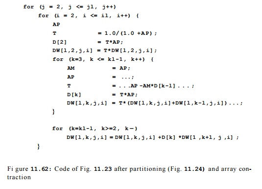
In the transformed multigrid program shown in Fig. 11.24, each
iteration of the inner loop produces and consumes a different element of AP,
AM, T, and a row of D. If these arrays are not used outside of the
code excerpt, the iterations can serially reuse the same data storage instead
of putting the values in different elements and rows, respectively. Figure
11.62 shows the result of reducing the dimensionality of the arrays. This code
runs faster than the original, because it reads and writes less data.
Especially in the case when an array is reduced to a scalar variable, we can
allocate the variable to a register and eliminate the need to access memory
altogether.
As less storage is
used, less parallelism is available. Iterations in the trans-formed code in
Fig. 11.62 now share data dependences and no longer can be executed in
parallel. To parallelize the code on P processors, we can expand
each of the scalar variables by a factor
of P and have each processor access its own private copy. Thus, the amount by which the storage is
expanded is
directly correlated
to the amount of parallelism exploited.
There are three reasons it is common to find opportunities for
array con-traction:
1.
Higher-level programming languages
for scientific applications, such as
Matlab and Fortran 90, support array-level operations. Each subexpres-sion of array
operations produces a temporary array. Because the arrays can be large, every
array operation such as a multiply or add would require reading and writing
many memory locations, while requiring relatively few arithmetic operations. It
is important that we reorder operations so that data is consumed as it is
produced and that we contract these arrays into scalar variables.
2. Supercomputers built in the 80's and 90's are all vector machines, so many scientific
applications developed then have been optimized for such machines. Even though
vectorizing compilers exist, many programmers still write their code to operate
on vectors at a time. The multigrid code example of this chapter is an example
of this style.
3. Opportunities for contraction are also introduced
by the compiler. As illustrated by variable T in the multigrid example,
a compiler would ex-pand arrays to improve parallelization. We have to contract
them when the space expansion is not necessary.
Example 1 T . 6 7 :
The array expression Z = W + X + Y translates to
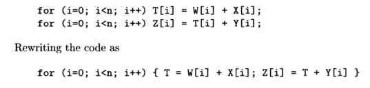
can speed it up considerably. Of course at the level of C code, we
would not even have to use the temporary T, but could write the assignment to Z[i]
as a single statement. However, here we are trying to model the
intermediate-code level at which a vector processor would deal with the
operations. •
A l g o r i t h m 1 1
. 6 8 : Array contraction.
INPUT: A program transformed by Algorithm 11.64.
OUTPUT: An equivalent program with reduced array
dimensions.
METHOD: A dimension of an array can be contracted to a
single element if
1. Each independent
partition uses only one element of the array,
2.
The value of
the element upon entry to the partition is not used by the partition, and
3.
The value of
the element is not live on exit from the partition.
Identify the contractable dimensions — those that satisfy the
three condi-tions above — and replace them with a single element. •
Algorithm 11.68 assumes that the program has first been
transformed by Al-gorithm 11.64 to pull all the dependent operations into a
partition and execute the partitions sequentially. It finds those array
variables whose elements' live ranges in different iterations are disjoint. If
these variables are not live after the loop, it contracts the array and has the
processor operate on the same scalar location. After array contraction, it may
be necessary to selectively expand arrays to accommodate for parallelism and
other locality optimizations.
The liveness analysis required here is more complex than that
described in Section 9.2.5. If the array is declared as a global variable, or
if it is a parameter, interprocedural analysis is required to ensure that the
value on exit is not used. Furthermore, we need to compute the liveness of
individual array elements, conservatively treating the array as a scalar would
be too imprecise.
Partition
Interleaving
Different partitions
in a loop often read the same data, or read and write the same cache lines. In
this and the next two sections, we discuss how to optimize for locality when
reuse is found across partitions.
R e u s e in
Innermost Blocks
We adopt the simple model that data can be found in the cache if
it is reused within a small number of iterations. If the innermost loop has a
large or un-known bound, only reuse across iterations of the innermost loop
translates into a locality benefit. Blocking creates inner loops with small known
bounds, al-lowing reuse within and across entire blocks of computation to be
exploited. Thus, blocking has the effect of capitalizing on more dimensions of
reuse.
E x a m p l e 1 1 . 6 9 :
Consider the matrix-multiply code shown in Fig. 11.5 and its blocked
version in Fig. 11.7. Matrix multiplication has reuse along every dimension of
its three-dimensional iteration space. In the original code, the in-nermost
loop has n iterations, where n is unknown and can be large. Our
simple model assumes that only the data reused across iterations in the
innermost loop is found in the cache.
In the blocked version, the three innermost loops execute a
three-dimension-al block of computation, with B iterations on each side.
The block size B is chosen by the compiler to be small enough so that
all the cache lines read and written within the block of computation fit into
the cache. Thus reused data across iterations in the third outermost loop can
be found in the cache. •
We refer to the innermost set of loops with small known bounds as
the inner-most block. It is desirable that the innermost block include
all the dimensions of the iteration space that carry reuse, if possible.
Maximizing the lengths of each side of the block is not as important. For the
matrix-multiply example, 3-dimensional blocking reduces the amount of data
accessed for each matrix by a factor of B2. If reuse is present, it is better to accommodate
higher-dimensional blocks with shorter sides than lower-dimensional blocks with
longer sides.
We can optimize locality of the innermost fully permutable loop
nest by blocking the subset of loops that share reuse. We can generalize the
notion of blocking to exploit reuses found among iterations of outer parallel
loops, also. Observe that blocking primarily interleaves the execution of a
small number of instances of the innermost loop. In matrix multiplication, each
instance of the innermost loop computes one element of the array answer; there
are n2 of them. Blocking interleaves the execution of a block of instances,
computing B iterations from each instance at a time. Similarly, we can
interleave iterations in parallel loops to take advantage of reuses between
them.
We define two primitives below that can reduce the distance
between reuses across different iterations. We apply these primitives
repeatedly, starting from the outermost loop until all the reuses are moved
adjacent to each other in the innermost block.
Interleaving Inner
Loops in a Parallel Loop
Consider the case
where an outer parallelizable loop contains an inner loop. To exploit reuse
across iterations of the outer loop, we interleave the executions of a fixed
number of instances of the inner loop, as shown in Fig. 11.63. Creating
two-dimensional inner blocks, this transformation reduces the distance between
reuse of consecutive iterations of the outer loop.
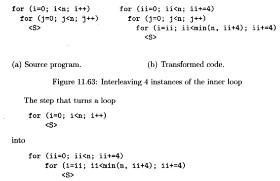
is known as stripmining. In the case where the outer loop
in Fig. 11.63 has a small known bound, we need not stripmine it, but can simply
permute the two loops in the original program.
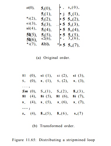
Interleaving S t a t
e m e n t s in a Parallel Loop
Consider the case where a parallelizable loop contains a sequence
of statements si, S2, • • • , sm. If some of these statements are loops themselves,
statements from consecutive iterations may still be separated by many
operations. We can exploit reuse between iterations by again interleaving their
executions, as shown in Fig. 11.64. This transformation distributes a
stripmined loop across the statements. Again, if the outer loop has a small
fixed number of iterations, we need not stripmine the loop but simply
distribute the original loop over all the statements.
We use Si(j) to denote the execution of
statement si in iteration j. Instead of the original sequential
execution order shown in Fig. 11.65(a), the code executes in the order shown in
Fig. 11.65(b).
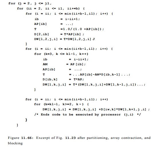
E x a m p l e 1 1 . 7 0 : We
now return to the multigrid example and show how we exploit reuse
between iterations of outer parallel loops. We observe that references DW[1,
k,j, i], DW[1, k-l,j,i], and DW[l,k+l,j,i]m the innermost loops of
the code in Fig. 11.62 have rather poor spatial locality. From reuse analysis,
as discussed in Section 11.5, the loop with index i carries spatial
locality and the loop with index k carries group reuse. The loop with
index k is already the innermost loop, so we are interested in
interleaving operations on DW from a block of partitions with
consecutive i values.
We apply the transform to interleave statements in the loop to
obtain the code in Fig. 11.66, then apply the transform to interleave inner
loops to obtain the code in Fig. 11.67. Notice that as we interleave B
iterations from loop with
index i, we
need to expand variables AP, AM,T into arrays that hold B results at a time. •
4. Putting it All Together
Algorithm 11.71 optimizes locality for a uniprocessor, and
Algorithm 11.72 optimizes both parallelism and locality for a multiprocessor.
A l g o r i t h m 1
1 . 7 1 : Optimize data locality on
a uniprocessor.
INPUT: A program with affine array accesses.
OUTPUT: An equivalent program that maximizes data
locality.
METHOD: Do the following steps:
1.
Apply Algorithm
11.64 to optimize the temporal locality of computed results.
2.
Apply Algorithm
11.68 to contract arrays where possible.
3.
Determine the
iteration subspace that may share the same data or cache lines using the
technique described in Section 11.5. For each statement, identify those outer
parallel loop dimensions that have data reuse.
4.
For each outer
parallel loop carrying reuse, move a block of the iterations into the innermost
block by applying the interleaving primitives repeat-edly.
5.
Apply blocking to the
subset of dimensions in the innermost fully per-mutable loop nest that carries
reuse.
6.
Block outer fully permutable
loop nest for higher levels of memory hier-archies, such as the third-level
cache or the physical memory.
7.
Expand scalars and arrays
where necessary by the lengths of the blocks.
•
A l g o r i t h m 1 1 . 7 2 :
Optimize parallelism and data locality for multiprocessors.
INPUT: A program with affine array accesses.
OUTPUT: An equivalent program that maximizes parallelism and data
locality.
METHOD: Do the following:
1. Use
the Algorithm 11.64 to parallelize the program and create an SPMD program.
2.
Apply Algorithm 11.71 to the SPMD program produced in Step 1 to optimize its locality.
5.
Exercises for Section 11.10
Exercise 11 . 10 . 1 : Perform array contraction on the following
vector operations:
for (i=0; i<n; i++)
T[i] = A[i] * B[i]; for (i=0; i<n; i++) D[i] = T[i] + C[i];
Exercise 11 . 10 . 2: Perform array
contraction on the following vector operations:
for (j = 2, j <= jl, j++)
for
(ii = 2, ii
<= il, ii+=b) {
for
(i = ii; i <=
min(ii+b-l,il); i++) {
ib = i-ii+1;
AP[ib] = ...;
T =1 . 0/(1 . 0
+AP[ib]);
D[2,ib] =
T*AP[ib] ;
DW[l,2,j,i] = T*DW[l,2,j,i]
;
}
for (k=3, k <= kl-1, k++)
for
(i = ii; i <=
min(ii+b-l,il); i++) {
ib = i-ii+1;
AM =
AP [ib];
AP[ib] = ...;
T =
. . .AP[ib]-AM*D[ib,k-l] . . .;
D[ib,k] =
T*AP;
DW[l,k,j,i] =
T*(DW[l,k,j,i]+DW[l,k-l,j,i])...;
}
for
(k=kl-l, k>=2,
k — ) {
for
(i = ii; i <=
min(ii+b-l,il); i++)
DW[l,k,j,i] = DW[l,k,j,i]
+D[iw,k]*DW[l,k+l,j,i] ;
/*
Ends code to be executed by processor (j,i)
*/
}
}
Figure 11.67: Excerpt of Fig. 11.23 after partitioning, array contraction,
and blocking
for (i=0; i<n; i++)
T[i] = A[i] + B[i]; for (i=0; i<n; i++) S[i] = C[i] + D[i]; for (i=0;
i<n; i++) E[i] = T[i] * S[i];
Exercise 1 1 . 1 0 . 3 :
Stripmine the outer loop
for (i=n-l; i>=0; i
— ) for (j=0; j<n; j++)
into strips of width 10.
Related Topics