Instruction Sets Prelimineris

INSTRUCTION SETS PRELIMINERIS:

1. Computer Architecture Taxonomy

                             Before we delve into the details of microprocessor instruction sets, it is helpful to develop some basic terminology. We do so by reviewing taxonomy of the basic ways we can organize a computer.

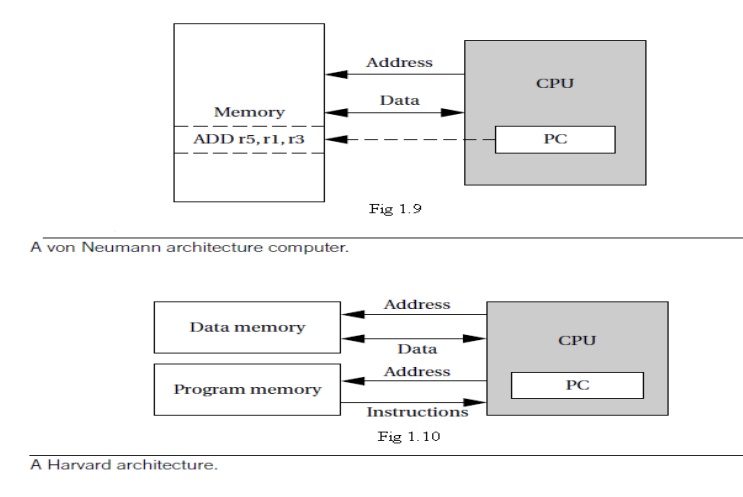
                             A block diagram for one type of computer is shown in Figure 1.9. The computing system consists of a central processing unit (CPU) and a memory.

                             The memory holds both data and instructions, and can be read or written when given an address. A computer whose memory holds both data and instructions is known as a von Neumann machine.

                             The CPU has several internal registers that store values used internally. One of those registers is the program counter (PC), which holds the address in memory of an instruction. The CPU fetches the instruction from memory, decodes the instruction, and executes it.

                             The program counter does not directly determine what the machine does next, but only indirectly by pointing to an instruction in memory. By changing only the instructions, we can change what the CPU does. It is this separation of the instruction memory from the CPU that distinguishes a stored-program computer from a general finite-state machine.

                             An alternative to the von Neumann style of organizing computers is the Harvard architecture, which is nearly as old as the von Neumann architecture. As shown in Figure 1.10, a Harvard machine has separate memories for data and program.

                             The program counter points to program memory, not data memory. As a result, it is harder to write self-modifying programs (programs that write data values, and then use those values as instructions) on Harvard machines.

                        Harvard architectures are widely used today for one very simple reason—the separation of program and data memories provides higher performance for digital signal processing.

                        Processing signals in real-time places great strains on the data access system in two ways: First, large amounts of data flow through the CPU; and second, that data must be processed at precise intervals, not just when the CPU gets around to it. Data sets that arrive continuously and periodically are called streaming data.

                        Having two memories with separate ports provides higher memory bandwidth; not making data and memory compete for the same port also makes it easier to move the data at the proper times. DSPs constitute a large fraction of all microprocessors sold today, and most of them are Harvard architectures.

                        A single example shows the importance of DSP: Most of the telephone calls in the world go through at least two DSPs, one at each end of the phone call.

                        Another axis along which we can organize computer architectures relates to their instructions and how they are executed. Many early computer architectures were what is known today as complex instruction set computers (CISC). These machines provided a variety of instructions that may perform very complex tasks, such as string searching; they also generally used a number of different instruction formats of varying lengths.

                             One of the advances in the development of high-performance microprocessors was the concept of reduced instruction set computers (RISC).These computers tended to provide somewhat fewer and simpler instructions.

                        The instructions were also chosen so that they could be efficiently executed in pipelined processors. Early RISC designs substantially outperformed CISC designs of the period. As it turns out, we can use RISC techniques to efficiently execute at least a common subset of CISC instruction sets, so the performance gap between RISC-like and CISC-like instruction sets has narrowed somewhat.

                        Beyond the basic RISC/CISC characterization, we can classify computers by several characteristics of their instruction sets. The instruction set of the computer defines the interface between software modules and the underlying hardware; the instructions define what the hardware will do under certain circumstances. Instructions can have a variety of characteristics, including:

                                                    Fixed versus variable length.

                                                    Addressing modes.

                                                    Numbers of operands.

                                                    Types of operations supported.

                        The set of registers available for use by programs is called the programming model, also known as the programmer model. (The CPU has many other registers that are used for internal operations and are unavailable to programmers.)

                        There may be several different implementations of architecture. In fact, the architecture definition serves to define those characteristics that must be true of all implementations and what may vary from implementation to implementation.

                        Different CPUs may offer different clock speeds, different cache configurations, changes to the bus or interrupt lines, and many other changes that can make one model of CPU more attractive than another for any given application.

2. Assembly Language

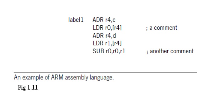
Figure 1.11 shows a fragment of ARM assembly code to remind us of the basic features of assembly languages. Assembly languages usually share the same basic features:

       One instruction appears per line.

       Labels, which give names to memory locations, start in the first column.

       Instructions must start in the second column or after to distinguish them from labels.

Comments run from some designated comment character (; in the case of ARM) to the end of the line.

                        Assembly language follows this relatively structured form to make it easy for the assembler to parse the program and to consider most aspects of the program line by line. ( It should be remembered that early assemblers were written in assembly language to fit in a very small amount of memory.

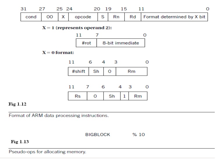
                        Those early restrictions have carried into modern assembly languages by tradition.) Figure 2.4 shows the format of an ARM data processing instruction such as an ADD.

ADDGT r0, r3, #5

                        For the instruction the cond field would be set according to the GT condition (1100), the opcode field would be set to the binary code for the ADD instruction (0100), the first operand register Rn would be set to 3 to represent r3, the destination register Rd would be set to 0 for r0, and the operand 2 field would be set to the immediate value of 5.

                        Assemblers must also provide some pseudo-ops to help programmers create complete assembly language programs.

                        An example of a pseudo-op is one that allows data values to be loaded into memory locations. These allow constants, for example, to be set into memory.

                        An example of a memory allocation pseudo-op for ARM is shown in Figure 2.5.TheARM % pseudo-op allocates a block of memory of the size specified by the operand and initializes those locations to zero.