Chapter: Compilers : Principles, Techniques, & Tools : Optimizing for Parallelism and Locality
Finding Synchronization-Free Parallelism
Finding Synchronization-Free Parallelism
1 An Introductory Example
2 Affine Space Partitions
3 Space-Partition Constraints
4 Solving Space-Partition
Constraints
5 A Simple Code-Generation
Algorithm
6 Eliminating Empty Iterations
7 Eliminating Tests from
Innermost Loops
8 Source-Code Transforms
9 Exercises for Section 11.7
Having developed the theory of affine array accesses, their reuse
of data, and the dependences among them, we shall now begin to apply this
theory to paral-lelization and optimization of real programs. As discussed in
Section 11.1.4, it is important that we find parallelism while minimizing
communication among processors. Let us start by studying the problem of
parallelizing an application without allowing any communication or synchronization
between processors at all. This constraint may appear to be a purely academic
exercise; how often can we find programs and routines that have such a form of
parallelism? In fact, many such programs exist in real life, and the algorithm
for solving this problem is useful in its own right. In addition, the concepts
used to solve this problem can be extended to handle synchronization and
communication.
1. An Introductory Example
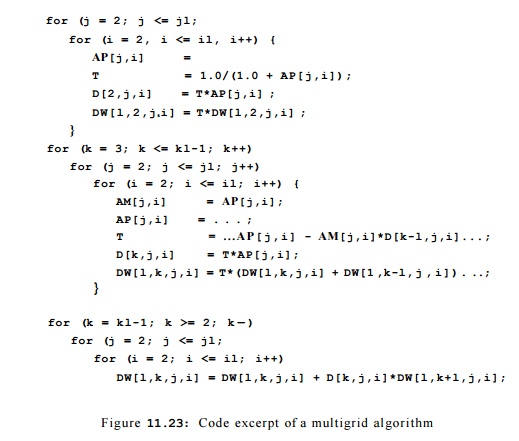
Shown in Fig. 11.23
is an excerpt of a C translation (with Fortran-style array accesses retained
for clarity) from a 5000-line Fortran multigrid algorithm to solve
three-dimensional Euler equations. The
program spends most its time in a small number of routines like the one shown
in the figure. It is typical of many numerical programs. These often consist of
numerous for-loops, with different nesting levels, and they have many array
accesses, all of which are affine expressions of surrounding loop indexes. To
keep the example short, we have elided lines from the original program with
similar characteristics.
The code of Fig. 11.23 operates on the scalar variable T
and a number of different arrays with different dimensions. Let us first
examine the use of variable T. Because each iteration in the loop uses
the same variable T, we cannot execute the iterations in parallel.
However, T is used only as a way to hold a common subexpression used
twice in the same iteration. In the first two of the three loop nests in Fig.
11.23, each iteration of the innermost loop writes a value into T and uses the
value immediately after twice, in the same iteration. We can eliminate the
dependences by replacing each use of T by the right-hand-side expression
in the previous assignment of T, without changing the semantics of the
program. Or, we can replace the scalar T by an array. We then have each
iteration use its own array element T[j, i].
With this
modification, the computation of an array element in each as-signment statement
depends only on other array elements with the same values for the last two
components (j and i, respectively). We can thus group all
operations that operate on the (j,i)th element of all arrays into
one computa-tion unit, and execute them in the original sequential order. This
modification produces ( j l — 1) x ( i l — 1) units of computation that are all
independent of one another. Notice that second and third nests in the source
program involve a third loop, with index k. However, because there is no
dependence between dynamic accesses with the same values for j and «, we
can safely perform the loops on k inside the loops on j and i
— that is, within a computation unit.
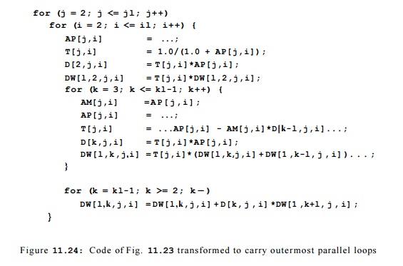
Knowing that these computation units are independent enables a
number of legal transforms on this code. For example, instead of executing the
code as originally written, a uniprocessor can perform the same computation by
execut-ing the units of independent operation one unit at a time. The resulting
code, shown in Fig. 11.24, has improved temporal locality, because results
produced are consumed immediately.
The independent units
of computation can also be assigned to different processors and executed in
parallel, without requiring any synchronization or communication. Since there
are ( j l — 1) x ( i l — 1) independent units of com putation, we can utilize at most ( j l - 1) x ( i
l - 1) processors. By organizing the processors as if they were in a
2-dimensional array, with ID's where 2
< j < jl
and 2 <
i < i l , the
SPMD program to be executed by
each processor is simply the body in the inner loop in Fig. 11.24.
The above example illustrates the basic approach to finding
synchronization-free parallelism. We first split the computation into as many
independent units as possible. This partitioning exposes the scheduling choices
available. We then assign computation units to the processors, depending on the
number of processors we have. Finally, we generate an SPMD program that is
executed on each processor.
2. Affine Space Partitions
A loop nest is said
to have k degrees of parallelism if it has, within the nest, k
parallelizable loops — that is, loops such that there are no data dependencies
between different iterations of the loops. For example, the code in Fig. 11.24 has 2 degrees of parallelism. It is convenient to
assign the operations in a com-putation with k degrees of parallelism to
a processor array with k dimensions.
We shall assume initially that each dimension of the processor array has as many
processors as there are iterations of the corresponding loop. After all the independent computation units have been found, we shall
map these "virtual" processors to the actual processors. In practice,
each processor should be responsible for a fairly large number of iterations,
because otherwise there is not enough work to amortize away the overhead of
parallelization.
We break down the
program to be parallelized into elementary statements, such as 3-address statements. For each statement, we find an affine
space partition that maps each dynamic instance of the statement, as
identified by its loop indexes, to a processor ID.
Example 1 1 . 4 0 :
As discussed above, the code of Fig. 11.23 has two degrees of parallelism. We
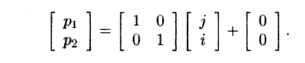
view the processor array as a 2-dimensional space. Let (pi,P2) be the ID of a
processor in the array. The parallelization scheme discussed in Section 11.7.1
can be described by simple affine partition functions. All the statements in
the first loop nest have this same affine partition:
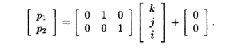
All the statements in
the second and third loop nests have the following same affine partition:
The algorithm to find
synchronization-free parallelism consists of three steps:
1.
Find, for each
statement in the program, an affine partition that maxi-mizes the degree of
parallelism. Note that we generally treat the state-ment, rather than the
single access, as the unit of computation. The same affine partition must apply
to each access in the statement. This grouping of accesses makes sense, since
there is almost always dependence among accesses of the same statement anyway.
2.
Assign the
resulting independent computation units among the processors, and choose an
interleaving of the steps on each processor. This assignment is driven by
locality considerations.
3.
Generate an
SPMD program to be executed on each processor.
We shall discuss next how to find the affine partition functions,
how to gen-erate a sequential program that executes the partitions serially,
and how to generate an SPMD program that executes each partition on a different
pro-cessor. After we discuss how parallelism with synchronizations is handled
in Sections 11.8 through 11.9.9, we return to Step 2 above in Section 11.10 and
discuss the optimization of locality for uniprocessors and multiprocessors.
3. Space-Partition Constraints
To require no communication, each pair of operations that share a
data depen-dence must be assigned to the same processor. We refer to these
constraints as "space-partition constraints." Any mapping that
satisfies these constraints cre-ates partitions that are independent of one
another. Note that such constraints can be satisfied by putting all the
operations in a single partition. Unfortu-nately, that "solution"
does not yield any parallelism. Our goal is to create as many independent
partitions as possible while satisfying the space-partition constraints; that
is, operations are not placed on the same processor unless it is necessary.
When we restrict ourselves to affine partitions, then instead of
maximizing the number of independent units, we may maximize the degree (number
of dimensions) of parallelism. It is sometimes possible to create more
independent units if we can use piecewise affine partitions. A piecewise
affine partition divides instances of a single access into, different sets and
allows a different affine partition for each set. However, we shall not
consider such an option here.
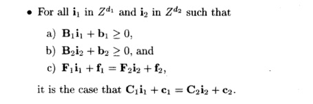
Formally, an affine
partition of a program is
synchronization free if and only if for every two (not necessarily
distinct) accesses sharing a dependence, T1
= ( F 1 , f 1 , B 1 , b 1 ) in statement s1 nested in d1 loops, and T2 = ( F 2 , f y , B 2 , b 2 ) in
statement s2 nested in d2 loops, the partitions ( C 1 , c 1 ) and ( C
2 , c 2 ) for statements si and s 2 , respectively, satisfy the following
space-partition constraints:
The goal of the parallelization algorithm is to find, for each
statement, the partition with the highest rank that satisfies these
constraints.
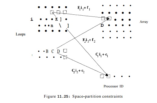
Shown in Fig. 11.25 is a diagram illustrating the essence of the
space-partition constraints. Suppose there are two static accesses in two loop
nests with index vectors ii and i 2 . These accesses are dependent in the
sense that they access at least one array element in common, and at least one
of them is a write. The figure shows particular dynamic accesses in the two
loops that hap pen to access
the same array element, according to the affine access functions Fiii + fi and
F 2 i 2 +f 2 . Synchronization is
necessary unless the affine partitions for the two static accesses, C i i i +
c i and C 2 i 2 + c 2 , assign the dynamic accesses to the same
processor.
If we choose an affine partition whose rank is the maximum of the
ranks of all statements, we get the maximum possible parallelism. However,
under this partitioning some processors may be idle at times, while other
processors are executing statements whose affine partitions have a smaller
rank. This situation may be acceptable if the time taken to execute those
statements is relatively short. Otherwise, we can choose an affine partition
whose rank is smaller than the maximum possible, as long as that rank is
greater than 0.
We show in Example
11.41 a small program designed to illustrate the power of the technique. Real
applications are usually much simpler than this, but may have boundary
conditions resembling some of the issues shown here. We shall use this example
throughout this chapter to illustrate that programs with
affine accesses have relatively simple space-partition
constraints, that these con-straints can be solved using standard linear
algebra techniques, and that the desired SPMD program can be generated
mechanically from the affine parti-tions.
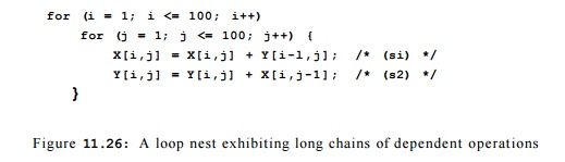
Example 1 1 . 4 1 :
This example shows how we formulate the space-partition constraints for the
program consisting of the small loop nest with two state-ments, si and s2, shown in Figure 11.26.
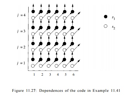
We show the data dependences in the program in Figure 1L27. That is, each black dot represents an instance of statement Si,
and each white dot represents a n instance o f statement S 2 . The dot
located a t coordinates (i, j ) represents the instance of the statement
that is executed for those values of the loop indexes.
Note, however, that the instance of s2 is located just below the
instance of «i for the same pair, so the vertical scale of j is greater than
the horizontal scale of i.
Notice that X[i,j] is written by si (i, j), that is, by the
instance of statement si with index values i and j. It is later read by s2(i,j
+ 1), so si(i,j) must precede s2(i,j + 1). This observation explains the
vertical arrows from black dots to white dots. Similarly, Y[i,j] is written by
s2(i,j) and later read by s1(i + 1, j). Thus, s2(i,j) must precede si(i + l,j),
which explains the arrows from white dots to black.
It is easy to see from this diagram that this code can be
parallelized without synchronization by assigning each chain of dependent
operations to the same processor. However, it is not easy to write the SPMD
program that implements this mapping scheme. While the loops in the original
program have 100 itera-tions each, there are 200 chains, with half originating
and ending with statement si and the other half originating and ending
with s2. The lengths of the chains vary from 1 to 100 iterations.
Since there are two statements, we are seeking two affine
partitions, one for each statement. We only need to express the space-partition
constraints for one-dimensional affine partitions. These constraints will be
used later by the solution method that tries to find all the independent
one-dimensional affine partitions and combine them to get multidimensional
affine partitions. We can thus represent the affine partition for each
statement by a 1 x 2 matrix and a 1 x 1
vector to translate the vector of indexes into a single processor
number. Let ([C11C12], [ci]), ([C2iC22], [c2 ]), be the one-dimensional affine
partitions for the statements s1 and
s2, respectively. We apply six data
dependence tests:
1. Write access
X[i,j] and itself in
statement si,
2. Write access X[i,j] with read access X[i, j] in
statement si,
3. Write access X[i,j]
in statement si with read access X[i,j — 1] in state-ment 82,
4. Write access ^ [ i
, j] and itself in statement s2,
5. Write access
Y[i,j] with read access Y[i,j] in statement s2,
6. Write access Y[i,
j] in statement s2 with read access Y[i
— l,j] in statement si .
We see that the dependence tests are all simple and highly
repetitive. The only dependences present in this code occur in case (3) between
instances of accesses
j] and X[i,j —
1] and in case (6) between Y[i,j] and Y[i — 1, j ] .
The space-partition
constraints imposed by the data dependence between
X[i,j] in statement si and X[i,j — 1] in statement
s2 can be expressed in the following terms:
For all and such that
1 < i < 100 1 < j < 100
1 < i' < 100 1 < j ' < 100
i = i'
we have
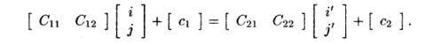
That is, the first
four conditions say that (i,j) and lie within the iteration space of the loop
nest, and the last two conditions say that the dynamic accesses X[i, j] and
X[i,j — 1] touch the same array
element. We can derive the
space-partition constraint for accesses Y[i — in statement s2 and Y[i, j] in
statement si in a similar manner.
4. Solving Space-Partition Constraints
Once the space-partition constraints have been extracted, standard
linear alge-bra techniques can be used to find the affine partitions satisfying
the constraints. Let us first show how we find the solution to Example 11.41.
Example 11 . 42 : We
can find the affine partitions for Example 11.41 with the following steps:
1.
Create the space-partition constraints
shown in Example 11.41. We use the loop bounds in determining the data
dependences, but they are not used in the rest of the algorithm otherwise.
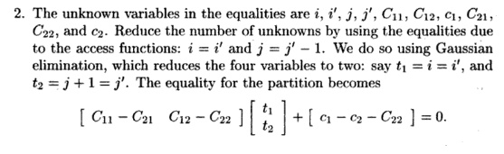
3. The equation above holds for all combinations of
t1 and t2- Thus, it must be that
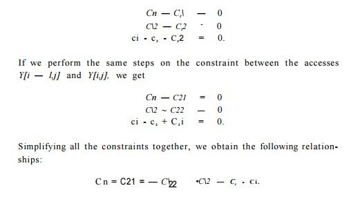
4.
Find all the independent solutions to
the equations involving only un-knowns in the coefficient matrix, ignoring the
unknowns in the constant vectors in this step. There is only one independent
choice in the coef-
ficient matrix, so
the affine partitions we seek can have at most a rank of one. We keep the
partition as simple as possible by setting Cn — 1. We cannot assign 0 to C11 because that will create a
rank-0 coefficient matrix, which maps all iterations to the same processor. It
then follows that C2i = 1, C22 = - 1, C12 = - 1 .
5. Find the constant
terms. We know that the difference between the constant terms, c2 — ci, must be
— 1 . We get to pick the actual values, however. To keep the partitions simple,
we pick c2 = 0; thus ci = — 1 .
Let p be the ID of the
processor executing iteration In terms of p, the affine partition is
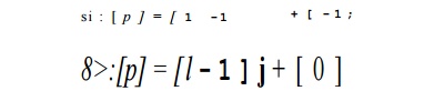
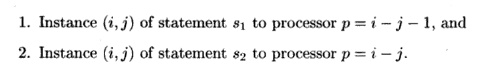
That is, the (i,j)th
iteration of si is assigned to the processor p = i — j — 1, and the (i,j)th
iteration of s2 is assigned to processor p — % — j.
Algorithm 11.43 :
Finding a highest-ranked synchronization-free affine partition for a program.
INPUT : A program with
affine array accesses.
OUTPUT : A partition.
METHOD : Do the following:
1. Find all
data-dependent pairs of accesses in a program for each pair of data-dependent
accesses, T1 — ( F i , f i , B i , b i )
in statement s1 nested in di loops
and T2 = ( F 2 , f 2 , B 2 , b 2
) in statement s2
nested in d2
loops. Let ( C i , c i ) and ( C 2 , c 2 ) represent the (currently
unknown) partitions of statements s1 and
s2, respectively. The space-partition constraints state

for all i1 and i2,
within their respective loop bounds. We shall generalize the domain of
iterations to include all ii in Zdl and i2 in Zd2;
that is, the bounds are all assumed to be minus infinity to infinity. This
assumption makes sense, since an affine partition cannot make use of the fact
that an index variable can take on only a limited set of integer values.
2. For each pair of
dependent accesses, we reduce the number of unknowns in the index vectors.
(a) Note
that Fi + f is the same vector as

That is, by adding an
extra component 1 at the bottom of column-vector i, we can make the
column-vector f be an additional, last column of the matrix F. We may thus
rewrite the equality of the access functions

(b) The above
equations will in general have more than one solution. However, we may still
use Gaussian elimination to solve the equations for the components of ix
and i2 as best we can. That is, eliminate as many variables as
possible until we are left with only variables that cannot be eliminated. The
resulting solution for i2 and i2 will have the form where
U is an upper-triangular matrix and t is a vector of free vari-ables ranging
over all integers.
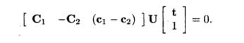
(c) We may use the
same trick as in Step (2a) to rewrite the equality of the partitions.
Substituting the vector (ii, i2 ,1) with the result
from Step (2b), we can write the constraints on the partitions as
3. Drop the
nonpartition variables. The equations above hold for all combi-nations of t if
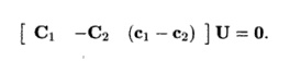
Rewrite these
equations in the form Ax = 0, where x is a vector of all the unknown
coefficients of the affine partitions.
4.
Find the rank of the affine partition
and solve for the coefficient matrices. Since the rank of an affine partition
is independent of the value of the constant terms in the partition, we
eliminate all the unknowns that come
from the constant
vectors like ci or c 2 , thus replacing Ax = 0 by sim-plified
constraints A'x' = 0. Find the solutions to A'x' = 0, expressing
them as B, a set of basis vectors spanning the null space of A'.
5.
Find the constant terms. Derive one
row of the desired affine partition from each basis vector in B, and derive the
constant terms using Ax = 0.
Note that Step 3
ignores the constraints imposed by the loop bounds on variables t. The
constraints are only stricter as a result, and the algorithm must therefore be
safe. That is, we place constraints on the C's and c's assuming t is arbitrary. Conceivably, there would be other
solutions for the C's and c's that are
valid only because some values of t are impossible. Not searching for these
other solutions may cause us to miss an optimization, but cannot cause the
program to be changed to a program that does something different from what the
original program does.
5. A Simple Code-Generation Algorithm
Algorithm 11.43 generates affine partitions that split
computations into inde-pendent partitions. Partitions can be assigned
arbitrarily to different proces-sors, since they are independent of one
another. A processor may be assigned more than one partition and can interleave
the execution of its partitions, as long as operations within each partition,
which normally have data dependences, are executed sequentially.
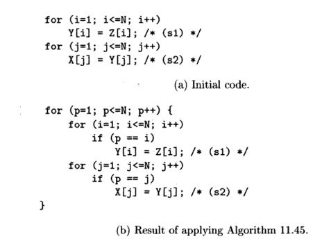
It is relatively easy to generate a correct program given an
affine partition. We first introduce Algorithm 11.45, a simple approach to generating code for a single processor that
executes each of the independent partitions sequentially. Such code optimizes
temporal locality, since array accesses that have several uses are very close
in time. Moreover, the code easily can be turned into an SPMD program that
executes each partition on a different processor. The code generated is,
unfortunately, inefficient; we shall next discuss optimizations to make the
code execute efficiently.
The essential idea is as follows. We are given bounds for the
index variables of a loop nest, and we have determined, in Algorithm 11.43, a partition for the accesses of a particular statement s.
Suppose we wish to generate sequential code that performs the action of each
processor sequentially. We create an outermost loop that iterates through the
processor IDs. That is, each iteration of this loop performs the operations
assigned to a particular processor ID. The original program is inserted as the
loop body of this loop; in addition, a test is added to guard each operation in
the code to ensure that each processor only executes the operations assigned to
it. In this way, we guarantee that the processor executes all the instructions
assigned to it, and does so in the original sequential order.
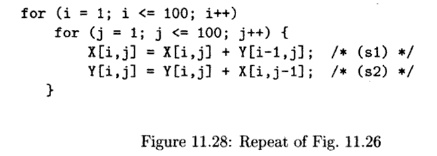
Example 11.44: Let us generate code that executes the
independent parti-tions in Example 11.41 sequentially. The original sequential program is
from Fig. 11.26 is repeated here as Fig. 11.28.
In Example 11.41, the affine partitioning algorithm found one
degree of parallelism. Thus, the processor space can be represented by a single
variable p. Recall also from that example that we selected an affine
partition that, for all values of index variables i and j
with 1 =< i =< 100 and 1 =< j =< 100, assigned
We can generate the
code in three steps:
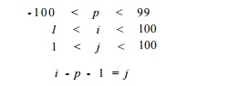
1.
For each statement, find all the
processor IDs participating in the com-putation. We combine the constraints 1 =< i =< 100 and 1 =< j =< 100 with one of the equations p = i - j - 1 or p = i - j, and project away i and j to
get the new constraints
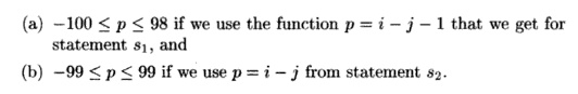
2. Find all the processor
IDs participating in any of the statements.
When
we take the union of
these ranges, we get - 1 0 0 =< p =< 99; these bounds
are sufficient to
cover all instances of both statements si and s 2 .
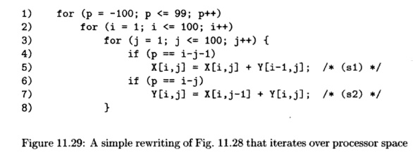
3.
Generate the
code to iterate through the computations in each partition sequentially. The
code, shown in Fig. 11.29, has an outer loop that iterates through all the
partition IDs participating in the computation (line (1)). Each partition goes
through the motion of generating the indexes of all the iterations in the
original sequential program in lines (2) and (3) so that it can pick out the
iterations the processor p is supposed to execute. The tests of lines
(4) and (6) make sure that statements s1 and s2 are executed
only when the processor p would execute them.
The generated code, while correct, is extremely inefficient.
First, even though each processor executes computation from at most 99
iterations, it gen-erates loop indexes for 100 x 100 iterations, an order of
magnitude more than necessary. Second, each addition in the innermost loop is
guarded by a test, creating another constant factor of overhead. These two
kinds of inefficiencies are dealt with in Sections 11.7.6 and 11.7.7,
respectively. •
Although the code of Fig. 11.29 appears designed to execute on a
unipro-cessor, we could take the inner loops, lines (2) through (8), and
execute them on 200 different processors, each of which had a different value
for p, from —100 to 99. Or, we could partition the responsibility for the
inner loops among any number of processors less than 200, as long as we
arranged that each processor knew what values of p it was responsible for and
executed lines (2) through (8) for just those values of p.
Algorithm 11.45 : Generating code that executes partitions of a
program sequentially.
INPUT : A program P with affine array accesses. Each statement s
in the program has associated bounds of the form B s i + bs > 0, where i is
the vector of loop indexes for the loop nest in which statement s appears.
Also associated with statement s is a partition C 5 i + cs = p
where p is an m-dimensional vector of variables representing a processor
ID; m is the maximum, over all statements in program P, of the
rank of the partition for that statement.
OUTPUT : A program equivalent to P but iterating over the
processor space over loop rather than indexes.
M E T H O D : Do the following:
1.
For each
statement, use Fourier-Motzkin elimination to project out all the loop index
variables from the bounds.
2.
Use Algorithm 11.13
to determine bounds on the partition ID's.
3. Generate loops, one for each of the m
dimensions of processor space. Let
p = [pi,P2, -- -
,Pm] be the vector of variables for these loops; that is, there is one
variable for each dimension of the processor space. Each loop variable pi
ranges over the union of the partition spaces for all statements in the program
P.
Note that the union of the partition spaces is not necessarily
convex. To keep the algorithm simple, instead of enumerating only those partitions
that
have a nonempty
computation to perform, set the lower
bound of each pi to
the minimum of all the lower bounds imposed by all statements and
the upper bound of each pi to the maximum of all the upper bounds
imposed by all statements. Some values of p may thereby have no
operations.
The code to be executed by each partition is the original
sequential pro-gram. However, every statement is guarded by a predicate so that
only those operations belonging to the partition are executed. •
An example of Algorithm 11.45 will follow shortly. Bear in mind,
however, that we are still far from the optimal code for typical examples.
6. Eliminating Empty Iterations
We now discuss the first of the two transformations necessary to
generate ef-ficient SPMD code. The code executed by each processor cycles
through all the iterations in the original program and picks out the operations
that it is supposed to execute. If the code has k degrees of
parallelism, the effect is that each processor performs k orders of
magnitude more work. The purpose of the first transformation is to tighten the
bounds of the loops to eliminate all the empty iterations.
We begin by considering the statements in the program one at a
time. A statement's iteration space to be executed by each partition is the
original itera-tion space plus the constraint imposed by the affine partition.
We can generate tight bounds for each statement by applying Algorithm 11.13 to
the new iter-ation space; the new index vector is like the original sequential
index vector, with processor ID's added as outermost indexes. Recall that the
algorithm will generate tight bounds for each index in terms of surrounding
loop indexes.
After finding the iteration spaces of the different statements, we
combine them, loop by loop, making the bounds the union of those for each
statement. Some loops end up having a single iteration, as illustrated by
Example 11.46 below, and we can simply eliminate the loop and simply set the
loop index to the value for that iteration.
Example 1 1 . 4 6
: For the loop of Fig. 11.30(a), Algorithm 11.43 will create the
affine partition

Algorithm 11.45 will create the code of Fig. 11.30(b). Applying
Algorithm 11.13 to statement s1 produces the bound: p < i < p,
or simply % = p. Similarly, the algorithm determines j = p
for statement s2- Thus, we get the code of Fig. 11.30(c). Copy propagation of
variables i and j will eliminate the unnec-essary test and
produce the code of Fig. 11.30(d). •
We now return to
Example 11.44 and illustrate the step to merge multiple iteration spaces from different statements together.
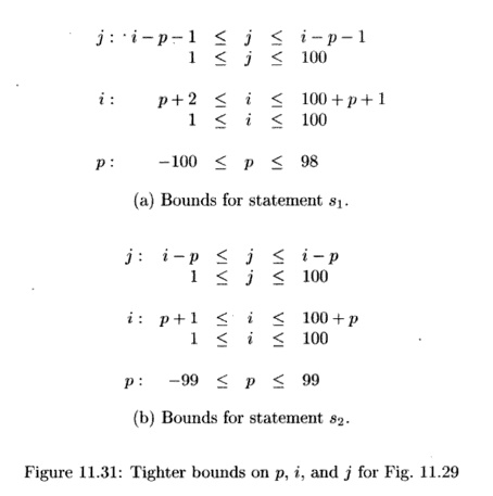
Example 11*47:
Let us now tighten the loop bounds of the code in Example 11.44. The
iteration space executed by partition p for statement si is defined by the
following equalities and inequalities:
Applying Algorithm 11.13 to the above creates the
constraints shown in Fig. 11.31(a). Algorithm 11.13 generates the constraint p
+ 2 < i < 100 + p + 1 from i — p - 1 = j and 1 < j < 100, and
tightens the upper bound of p to 98.
Likewise, the bounds for each of the variables for
statement s2 are shown in Fig. 11.31(b).
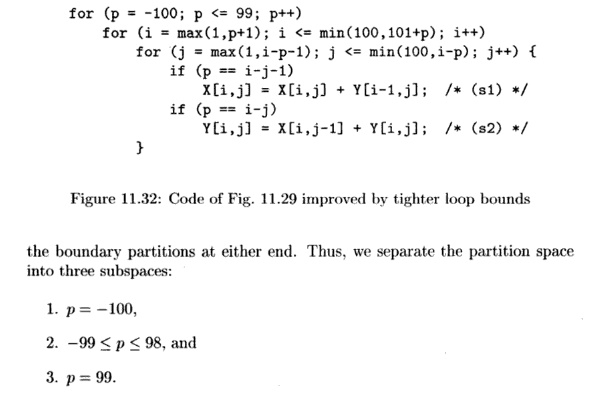
The iteration spaces
for si and s2 in Fig. 11.31 are similar, but as
ex-pected from Fig. 11.27, certain limits differ by 1 between the two. The code
in Fig. 11.32 executes over this union of iteration spaces. For example, for i
use min(l,£>+1) as the lower bound and max(100,100+ p + 1 ) as the upper
bound. Note that the innermost loop has 2 iterations except that it has only
one the first and last time it is executed. The overhead in generating loop
indexes is thus reduced by an order of magnitude. Since the iteration space
executed is larger than either that of si
and s2, conditionals are still necessary to select when these
statements are executed.

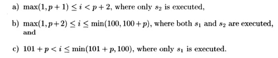
7. Eliminating Tests from Innermost Loops
The second transformation is to remove conditional tests from the
inner loops. As seen from the examples above, conditional tests remain if the
iteration spaces of statements in the loop intersect but not completely. To
avoid the need for conditional tests, we split the iteration space into
subspaces, each of which executes the same set of statements. This optimization
requires code to be duplicated and should only be used to
remove conditionals in the inner loops.
To split an iteration
space to reduce tests in inner loops, we apply the following steps repeatedly
until we remove all the tests in the inner loops:
1. Select a loop that consists of statements with
different bounds.
2.
Split the loop using a condition such
that some statement is excluded from at least one of its components. We choose
the condition from among the boundaries of the overlapping different polyhedra.
If some statement has all its iterations in only one of the half planes of the
condition, then such a condition is useful.
3. Generate code for
each of these iteration spaces separately.
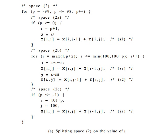
Example 1 1 . 4 8 : Let
us remove the conditionals from the code of Fig. 11.32. Statements si and 52 are mapped to the same set of
partition ID's except for
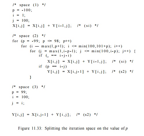
The code for each
subspace can then be specialized for the value(s) of p contained. Figure
11.33 shows the resulting code for each of
the three iteration
spaces.
Notice that the first
and third spaces do not need loops on i or j, because for the particular
value of p that defines each space, these loops are degenerate; they
have only one iteration. For example, in space (1), substituting p = —100 in the loop bounds restricts i to 1, and subsequently j to 100. The assignments
to p in spaces (1) and (3) are evidently
dead code and can be eliminated.
Next we split the
loop with index i in space (2). Again, the first and last iterations of loop index i are
different. Thus, we split the loop into three subspaces:
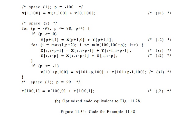
The loop nest for
space (2) in Fig. 11.33 can thus be written as in Fig. 11.34(a). Figure 11.34(b) shows the optimized program. We have substituted Fig.
11.34(a) for the loop nest in Fig. 11.33. We also propagated out assignments to
p, i, and j into the array accesses.
When optimizing at the intermediate-code level, some of these
assignments will be identified as common subexpressions and re-extracted from
the array-access code.
8. Source-Code Transforms
We have seen how we can derive from simple affine partitions for
each statement programs that are significantly different from the original
source. It is not apparent from the examples seen so far how affine partitions
correlate with changes at the source level. This section shows that we can
reason about source code changes relatively easily by breaking down affine
partitions into a series of primitive transforms.
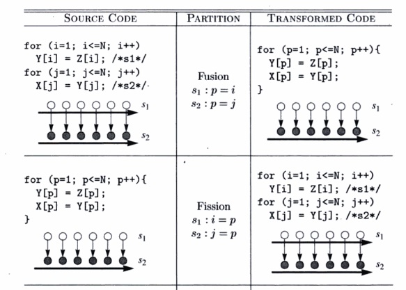
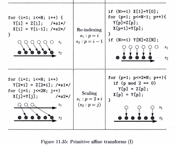
Seven Primitive Affine Transforms
Every affine partition can be expressed as a series of primitive
affine transforms, each of which corresponds to a simple change at the source
level. There are seven kinds of primitive transforms: the first four primitives
are illustrated in Fig. 11.35, the last three, also known as unimodular
transforms, are illustrated in Fig. 11.36.
The figure shows one example for each primitive: a source, an
affine parti-tion, and the resulting code. We also draw the data dependences
for the code before and after the transforms. From the data dependence
diagrams, we see that each primitive corresponds to a simple geometric
transform and induces a relatively simple code transform. The seven primitives
are:
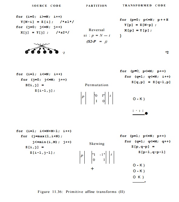
Unimodular Transforms
A unimodular transform is represented by just a unimodular
coefficient matrix and no constant vector. A unimodular matrix is a
square matrix whose determinant is ± 1 . The significance of a unimodular
transform is that it maps an n-dimensional iteration space to another
n-dimensional polyhedron, where there is a one-to-one correspondence between
iterations of the two spaces.
1.
Fusion. The fusion transform is characterized by mapping
multiple loop indexes in the original program to the same loop index.
The new loop fuses statements from different loops.
2. Fission. Fission is the inverse of fusion. It maps the same
loop index for different statements to different loop indexes in the
transformed code. This splits the original loop into multiple loops.
3. Re-indexing. Re-indexing shifts the dynamic executions of a
statement by a constant number of iterations. The affine transform has a
constant term.
4.
Scaling. Consecutive iterations in the source program are
spaced apart by a constant factor. The affine transform has a positive
nonunit coefficient.
5.
Reversal. Execute iterations in a loop in reverse order. Reversal
is char-acterized by having —1 as a coefficient.
6.
Permutation. Permute the inner and outer loops. The affine
transform consists of permuted rows of the identity matrix.
7.
Shewing. Iterate through the iteration space in the loops
at an angle. The affine transform is a unimodular matrix with l's on the
diagonal.
A Geometric Interpretation of Parallelization
The affine transforms shown in all but the fission example are
derived by apply-ing the synchronization-free affine partition algorithm to the
respective source codes. (We shall discuss how fission can parallelize code
with synchronization in the next section.) In each of the examples, the
generated code has an (outer-most) parallelizable loop whose iterations can be
assigned to different processors and no synchronization is necessary.
These examples illustrate that there is a simple geometric
interpretation of how parallelization works. Dependence edges always point from
an earlier instance to a later instance. So, dependences between separate statements
not nested in any common loop follows the lexical order; dependences between statements nested in the same loop follows the
lexicographic order. Geometri-cally, dependences of a two-dimensional loop nest
always point within the range [0°, 180°), meaning that the angle of the
dependence must be below 180°, but no less than 0°.
The affine transforms change the ordering of iterations such that
all the dependences are found only between operations nested within the same
iteration of the outermost loop. In other words, there are no dependence edges
at the boundaries of iterations in the outermost loop. We can parallelize
simple source codes by drawing their dependences and finding such transforms
geometrically.
9. Exercises for Section 11.7
Exercise 1 1 . 7 . 1 : For the
following loop
for (i = 2;
i < 100; i++)
A[i] =
A[i-2];
a)
What is the
largest number of processors that can be used effectively to execute this loop?
b)
Rewrite the
code with processor p as a parameter.
c)
Set up and find
one solution to the space-partition constraints for this loop.
d) What is the affine partition of highest rank
for this loop?
Exercise 11 . 7 . 2: Repeat Exercise 11.7.1 for the loop nests in Fig.
11.37.
Exercise 11 . 7 .
3: Rewrite the following code
for
(i = 0; i < 100; i++) A[i] = 2*A[i] ;
for
(j = 0; j < 100; j++) A[j] = A[j] + 1;
so it consists of a single loop. Rewrite the loop in terms of a
processor number p so the code can be partitioned among 100 processors,
with iteration p executed by processor p.
Exercise 11 . 7 .
4: In the following code
for (i = 1;
i < 100; i++)
for (j =
1; j
< 100; j++)
/* (s) */ A[i,j] =
(A[i-l,j] + A[i+l,j]
+ A[i,j-1] + A[i,j+l])/4;
for (i = 0; i <= 97;
i++)
A[i] = A[i+2] ;
(a)
for (i = 1; i <= 100;
i++)
for (j = 1; j <=
100; j++)
for (k = 1; k <= 100; k++) {
A[i,j,k] = A[i,j,k]
+ B[i-l,j,k];
B[i,j,k] = B[i,j,k] +
C[i, j-l,k] ;
C[i,j,k] =
C[i,j,k] + A[i,j,k-1];
}
!(b)
for (i = 1; i <= 100;
i++)
for (j = 1;
j <= 100; j++)
for (k = 1; k <=
100; k++) {
A[i,j,k] = A[i,j,k]
+ B[i-l,j,k];
B[i,j,k] = B[i,j,k]
+ A[i,j-l,k];
C[i,j,k] =
C[i,j,k] + A[i,j,k-1] + B[i,j,k];
}
!(c)
Figure 11.37: Code for Exercise 11.7.2
the only constraints
are that the statement s that forms the body of the loop
nest must execute
iterations s(i — l,j) and s(i, j — 1) before executing iteration
s(i,j). Verify that
these are the only necessary constraints. Then rewrite the code so that
the outer loop has index variable p, and on the pth iteration of the outer
loop, all instances of s(i,j) such that i + j = p are executed.
Exercise
1 1 . 7 . 5 : Repeat Exercise 11.7.4, but arrange that on the pth iteration of the outer loop, instances of s such that i — j = p
are executed.
! Exercise 1 1 . 7 . 6 : Combine the following loops
for
(i = 0; i < 100; i++) A[i] = B[i];
for
(j = 98; j >= 0; j = j-2) B[i] = i;
into a single loop, preserving all dependencies.
Exercise 11 . 7 . 7: Show
that the matrix
is unimodular. Describe the transformation it performs on a
two-dimensional loop nest.
Exercise 11 . 7 . 8: Repeat
Exercise 11.7.7 on the matrix
Related Topics