Three Dimensional Object Representations

Three Dimensional Object Representations

Representation schemes for solid objects are divided into two categories as follows: 1. Boundary Representation ( B-reps)

It describes a three dimensional object as a set of surfaces that separate the object interior from the environment. Examples are polygon facets and spline patches.

2. Space Partitioning representation

It describes the interior properties, by partitioning the spatial region containing an object into a set of small, nonoverlapping, contiguous solids(usually cubes). Eg: Octree Representation.

Polygon Surfaces

Polygon surfaces are boundary representations for a 3D graphics object is a set of polygons that enclose the object interior.

Polygon Tables

The polygon surface is specified with a set of vertex coordinates and associated attribute parameters.

For each polygon input, the data are placed into tables that are to be used in the subsequent processing.

Polygon data tables can be organized into two groups: Geometric tables and attribute tables.

Geometric Tables Contain vertex coordinates and parameters to identify the spatial orientation of the polygon surfaces.

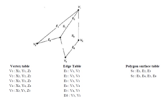
Attribute tables Contain attribute information for an object such as parameters specifying the degree of transparency of the object and its surface reflectivity and texture characteristics. A convenient organization for storing geometric data is to create three lists:

1. The Vertex Table

Coordinate values for each vertex in the object are stored in this table. 2. The Edge Table

It contains pointers back into the vertex table to identify the vertices for each polygon edge. 3. The Polygon Table

It contains pointers back into the edge table to identify the edges for each polygon. This is shown in fig

Listing the geometric data in three tables provides a convenient reference to the individual components (vertices, edges and polygons) of each object.

The object can be displayed efficiently by using data from the edge table to draw the component lines.

Extra information can be added to the data tables for faster information extraction. For instance, edge table can be expanded to include forward points into the polygon table so that common edges between polygons can be identified more rapidly.

E1 : V1, V2, S1

E2 : V2, V3, S1

E3 : V3, V1, S1, S2

E4 : V3, V4, S2

E5 : V4, V5, S2

E6 : V5, V1, S2

is useful for the rendering procedure that must vary surface shading smoothly across the edges from one polygon to the next. Similarly, the vertex table can be expanded so that vertices are cross-referenced to corresponding edges.

Additional geometric information that is stored in the data tables includes the slope for each edge and the coordinate extends for each polygon. As vertices are input, we can calculate edge slopes and we can scan the coordinate values to identify the minimum and maximum x, y and z values for individual polygons.

The more information included in the data tables will be easier to check for errors. Some of the tests that could be performed by a graphics package are:

1. That every vertex is listed as an endpoint for at least two edges.

2. That every edge is part of at least one polygon.

3. That every polygon is closed.

4. That each polygon has at least one shared edge.

5.  That if the edge table contains pointers to polygons, every edge referenced by a polygon pointer has a reciprocal pointer back to the polygon.

Plane Equations:

To produce a display of a 3D object, we must process the input data representation for the object through several procedures such as,

-  Transformation of the modeling and world coordinate descriptions to viewing coordinates.

-  Then to device coordinates:

-  Identification of visible surfaces

-  The application of surface-rendering procedures.

For these processes, we need information about the spatial orientation of the individual surface components of the object. This information is obtained from the vertex coordinate value and the equations that describe the polygon planes.

The equation for a plane surface is Ax + By+ Cz + D = 0 ----(1)

Where (x, y, z) is any point on the plane, and the coefficients A,B,C and D are constants describing the spatial properties of the plane.

We can obtain the values of A, B,C and D by solving a set of three plane equations using the coordinate values for three non collinear points in the plane.

For that, we can select three successive polygon vertices (x1, y1, z1), (x2, y2, z2) and (x3, y3, z3) and solve the following set of simultaneous linear plane equations for the ratios A/D, B/D and C/D.

(A/D)xk + (B/D)yk + (c/D)zk = -1, k=1,2,3 -----(2)

The solution for this set of equations can be obtained in determinant form, using Cramer’s rule as

Expanding the determinants , we can write the calculations for the plane coefficients in the form: 

A = y1 (z2 –z3 ) + y2(z3 –z1 ) + y3 (z1 –z2 )

B = z1 (x2 -x3 ) + z2 (x3 -x1 ) + z3 (x1 -x2 )

C = x1 (y2 –y3 ) + x2 (y3 –y1 ) + x3 (y1 -y2 )

D = -x1 (y2 z3 -y3 z2 ) - x2 (y3 z1 -y1 z3 ) - x3 (y1 z2 -y2 z1) ------(4)

As vertex values and other information are entered into the polygon data structure, values for A, B, C and D are computed for each polygon and stored with the other polygon data.

Plane equations are used also to identify the position of spatial points relative to the plane surfaces of an object. For any point (x, y, z) hot on a plane with parameters A,B,C,D, we have

Ax + By + Cz + D ≠ 0

We can identify the point as either inside or outside the plane surface according o the sigh (negative or positive) of Ax + By + Cz + D:

If Ax + By + Cz + D < 0, the point (x, y, z) is inside the surface. If Ax + By + Cz + D > 0, the point (x, y, z) is outside the surface.

These inequality tests are valid in a right handed Cartesian system, provided the plane parmeters A,B,C and D were calculated using vertices selected in a counter clockwise order when viewing the surface in an outside-to-inside direction.

Polygon Meshes

A single plane surface can be specified with a function such as fillArea. But when object surfaces are to be tiled, it is more convenient to specify the surface facets with a mesh function. One type of polygon mesh is the triangle strip.A triangle strip formed with 11 triangles connecting 13 vertices.

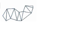
This function produces n-2 connected triangles given the coordinates for n vertices.

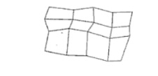
Another similar function in the quadrilateral mesh, which generates a mesh of (n-1) by (m-1) quadrilaterals, given the coordinates for an n by m array of vertices. Figure shows 20 vertices forming a mesh of 12 quadrilaterals.

Curved Lines and Surfaces Displays of three dimensional curved lines and surface can be generated from an input set of mathematical functions defining the objects or from a set of user specified data points. When functions are specified, a package can project the defining equations for a curve to the display plane and plot pixel positions along the path of the projected function. For surfaces, a functional description in decorated to produce a polygon-mesh approximation to the surface.

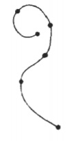
Spline Representations A Spline is a flexible strip used to produce a smooth curve through a designated set of points. Several small weights are distributed along the length of the strip to hold it in position on the drafting table as the curve is drawn.

The Spline curve refers to any sections curve formed with polynomial sections satisfying specified continuity conditions at the boundary of the pieces.

A Spline surface can be described with two sets of orthogonal spline curves. Splines are used in graphics applications to design curve and surface shapes, to digitize drawings for computer storage, and to specify animation paths for the objects or the camera in the scene. CAD applications for splines include the design of automobiles bodies, aircraft and spacecraft surfaces, and ship hulls.

Interpolation and Approximation Splines Spline curve can be specified by a set of coordinate positions called control points which indicates the general shape of the curve. These control points are fitted with piecewise continuous parametric polynomial functions in one of the two ways. 1. When polynomial sections are fitted so that the curve passes through each control point the resulting curve is said to interpolate the set of control points.

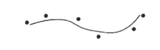
A set of six control points interpolated with piecewise continuous polynomial sections

1. When the polynomials are fitted to the general control point path without necessarily passing through any control points, the resulting curve is said to approximate the set of control points.

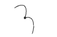
A set of six control points approximated with piecewise continuous polynomial sections

Interpolation curves are used to digitize drawings or to specify animation paths. Approximation curves are used as design tools to structure object surfaces. A spline curve is designed , modified and manipulated with operations on the control points.The curve can be translated, rotated or scaled with transformation applied to the control points. The convex polygon boundary that encloses a set of control points is called the convex hull. The shape of the convex hull is to imagine a rubber band stretched around the position of the control points so that each control point is either on the perimeter of the hull or inside it. Convex hull shapes (dashed

lines) for two sets of control points

Parametric Continuity Conditions

For a smooth transition from one section of a piecewise parametric curve to the next various continuity conditions are needed at the connection points.

If each section of a spline in described with a set of parametric coordinate functions or the form x = x(u), y = y(u), z = z(u), u1<= u <= u2 -----(a)

We set parametric continuity by matching the parametric derivatives of adjoining curve sections at their common boundary.

Zero order parametric continuity referred to as C0 continuity, means that the curves meet. (i.e) the values of x,y, and z evaluated at u2 for the first curve section are equal. Respectively, to the value of x,y, and z evaluated at u1 for the next curve section.

First order parametric continuity referred to as C1 continuity means that the first parametric derivatives of the coordinate functions in equation (a) for two successive curve sections are equal at their joining point.

Second order parametric continuity, or C2 continuity means that both the first and second parametric derivatives of the two curve sections are equal at their intersection.

Higher order parametric continuity conditions are defined similarly.

Piecewise construction of a curve by joining two curve segments using different orders of continuity

a)Zero order continuity only

b)First order continuity only

c) Second order continuity only

Geometric Continuity Conditions

To specify conditions for geometric continuity is an alternate method for joining two successive curve sections.

The parametric derivatives of the two sections should be proportional to each other at their common boundary instead of equal to each other.

Zero order Geometric continuity referred as G0 continuity means that the two curves sections must have the same coordinate position at the boundary point.

First order Geometric Continuity referred as G1 continuity means that the parametric first derivatives are proportional at the interaction of two successive sections.

Second order Geometric continuity referred as G2 continuity means that both the first and second parametric derivatives of the two curve sections are proportional at their boundary. Here the curvatures of two sections will match at the joining position.

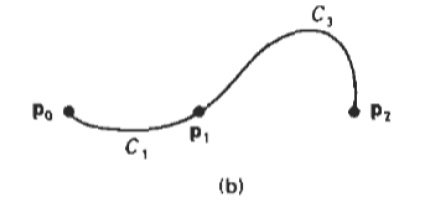
Three control points fitted with two curve sections joined with a) parametric continuity

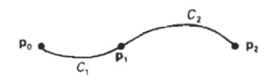
b)geometric continuity where the tangent vector of curve C3 at point p1 has a greater magnitude than the tangent vector of curve C1 at p1.

Spline specifications There are three methods to specify a spline representation:

1. We can state the set of boundary conditions that are imposed on the spline; (or)

2. We can state the matrix that characterizes the spline; (or)

3. We can state the set of blending functions that determine how specified geometric constraints on the curve are combined to calculate positions along the curve path.

To illustrate these three equivalent specifications, suppose we have the following parametric cubic polynomial representation for the x coordinate along the path of a spline section.

x(u)=axu3 + axu2 + cxu + dx 0<= u <=1 ----------(1) Boundary conditions for this curve might be set on the endpoint coordinates x(0) and x(1) and on the parametric first derivatives at the endpoints x’(0) and x’(1). These boundary conditions are sufficient to determine the values of the four coordinates ax, bx, cx and dx. From the boundary conditions we can obtain the matrix that characterizes this spline curve by first rewriting eq(1) as the matrix product

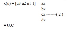
where U is the row matrix of power of parameter u and C is the coefficient column matrix. Using equation (2) we can write the boundary conditions in matrix form and solve for the coefficient matrix C as

C = Mspline . Mgeom -----(3) Where Mgeom in a four element column matrix containing the geometric constraint values on the spline and Mspline in the 4 * 4 matrix that transforms the geometric constraint values to the polynomial coefficients and provides a characterization for the spline curve.

Matrix Mgeom contains control point coordinate values and other geometric constraints. We can substitute the matrix representation for C into equation (2) to obtain.

x (u) = U . Mspline . Mgeom ------(4)

The matrix Mspline, characterizing a spline representation, called the basis matriz is useful for transforming from one spline representation to another.

Finally we can expand equation (4) to obtain a polynomial representation for coordinate x in terms of the geometric constraint parameters.

x(u) = Σ gk. BFk(u) where gk are the constraint parameters, such as the control point coordinates and slope of the curve at the control points and BFk(u) are the polynomial blending functions.