Chapter: Operations Research: An Introduction : The Simplex Method and Sensitivity Analysis
The Simplex Method
THE SIMPLEX METHOD
Rather than enumerating all the basic solutions (corner points) of the LP problem (as we did in previous pages), the simplex method investigates only a "select few" of these solutions. Section 1 describes the iterative nature of the method, and Section 2 provides the computational details of the simplex algorithm.
1. Iterative Nature of the Simplex Method
Figure 3.3 provides the solution space of the LP of Example 3.2-1. Normally, the sim-plex method starts at the origin (point A) where xl = x2 = O. At this starting point, the value of the objective function, z, is zero, and the logical question is whether an increase in nonbasic xl and/or x2 above their current zero values can improve (increase) the value of z. We answer this question by investigating the objective function:
Maximize z = 2x1 + 3x2
The function shows that an increase in either xl or x2 (or both) above their current zero values will improve the value of z. The design of the simplex method calls for in-creasing one variable at a time, with the selected variable being the one with the largest
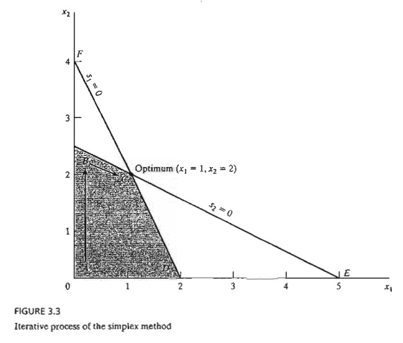
rate of improvement in z. In the present example, the value of z will increase by 2 for each unit increase in xl and by 3 for each unit increase in x2. This means that the rate of improvement in the value of z is 2 for xl and 3 for x2. We thus elect to increase x2, the variable with the largest rate of improvement. Figure 3.3 shows that the value of x2 must be increased until corner point B is reached (recall that stopping short of reaching corner point B is not optimal because a candidate for the optimum must be a corner point). At point B, the simplex method will then increase the value of xl to reach the improved corner point C, which is the optimum. The path of the simplex algorithm is thus defined as A - > B -> C. Each corner point along the path is associated with an iteration. It is important to note that the simplex method moves alongside the edges of the solution space, which means that the method cannot cut across the solution space, going from A to C directly.
We need to make the transition from the graphical solution to the algebraic solu-tion by showing how the points A, B, and C are represented by their basic and nonba-sic variables. The following table summarizes these representations:
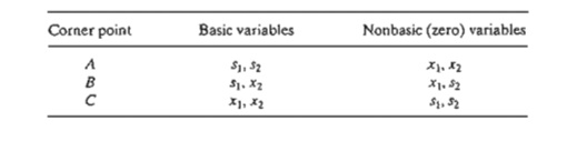
Notice the change pattern in the basic and nonbasic variables as the solution moves along the path A -> B -> C. From A to B, nonbasic x2 at A becomes basic at Band basic s2 at A becomes nonbasic at B. In the terminology of the simplex method, we say that x2 is the entering variable (because it enters the basic solution) and s2 is the leaving variable (because it leaves the basic solution). In a similar manner, at point B, xl enters (the basic solution) and sl leaves, thus leading to point C.
PROBLEM SET 3.3A
1. In Figure 3.3, suppose that the objective function is changed to
Maximize z = 8x1 + 4x2
Identify the path of the simplex method and the basic and nonbasic variables that define this path.
2. Consider the graphical solution of the Reddy Mikks model given in Figure 2.2. Identify the path of the simplex method and the basic and nonbasic variables that define this path.
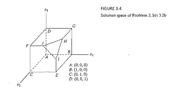
*3. Consider the three-dimensional LP solution space in Figure 3.4, whose feasible extreme points are A, B, ... , and J.
a.Which of the following pairs of corner points cannot represent successive simplex iterations: (A, B), (B, D), (E, H), and (A, I)? Explain the reason.
b.Suppose that the simplex iterations start at A and that the optimum occurs at H. Indicate whether any of the following paths are not legitimate for the simplex algorithm, and state the reason.
A -> B -> G -> H .
A -> E -> I -> H .
A -> C -> E -> B -> A -> D -> G -> H .
4. For the solution space in Figure 3.4, all the constraints are of the type ≤ and all the variables x1, x2, and x3 are nonnegative. Suppose that s1, s2, s3, and s4 (≥ 0) are the slacks associated with constraints represented by the planes CElJF, BEIHG, DFJHG, and IJH, respectively. Identify the basic and nonbasic variables associated with each feasible ex-treme point of the solution space.
5. Consider the solution space in Figure 3.4, where the simplex algorithm starts at point A.
Determine the entering variable in the first iteration together with its value and the improvement in z for each of the following objective functions:
Maximize z = xI – 2x2 + 3x3
Maximize z = 5x1 + 2x2 + 4x3
Maximize z = -2xI + 7x2 + 2x3
Maximize z = xl + x2 + x3
2. Computational Details of the Simplex Algorithm
This section provides the computational details of a simplex iteration, including the rules for determining the entering and leaving variables as well as for stopping the computations when the optimum solution has been reached. The vehicle of explana-tion is a numerical example.
Example 3.3-1
We use the Reddy Mikks model (Example 2.1-1) to explain the details of the simplex method. The problem is expressed in equation form as
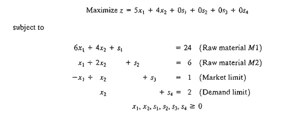
The variables s1 s2, s3, and s4 are the slacks associated with the respective constraints. Next, we write the objective equation as
z-5x1-4x2=0
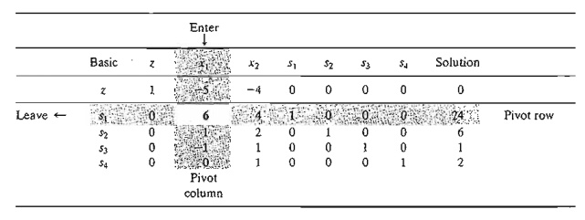
In this manner, the starting simplex tableau can be represented as follows:
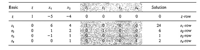
The design of the tableau specifies the set of basic and nonbasic variables as well as provides the solution associated with the starting iteration. As explained in Section 3.3.1, the simplex iterations start at the origin (xl, x2) = (0,0) whose associated set of nonbasic and basic variables are defined as
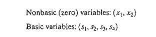
Substituting the nonbasic variables (x1 , x2) = (0,0) and noting the special 0-1 arrangement of the coefficients of z and the basic variables (s1, s2, s3,s4) in the tableau, the following solution is immediately available (without any calculations):
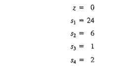
This information is shown in the tableau by listing the basic variables in the leftmost Basic column and their values in the rightmost Solution column. In effect, the tableau defines the current corner point by specifying its basic variables and their values, as well as the corresponding value of the objective function, z. Remember that the nonbasic variables (those not listed in the Basic column) always equal zero.
Is the starting solution optimal? The objective function z = 5xl + 4x2 shows that the solution can be improved by increasing xl or x2. Using the argument in Section 3.3.1, xl with the most positive coefficient is selected as the entering variable. Equivalently, because the simplex tableau expresses the objective function as z - 5x1 - 4x2 = 0, the entering variable will correspond to the variable with the most negative coefficient in the objective equation. This rule is referred to as the optimality condition.
The mechanics of determining the leaving variable from the simplex tableau calls for com-puting the nonnegative ratios of the right-hand side of the equations (Solution column) to the corresponding constraint coefficients under the entering variable, xl, as the following table shows.
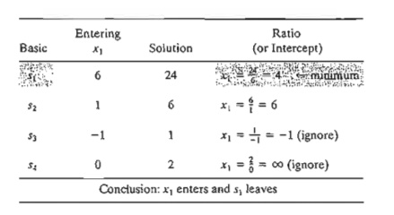
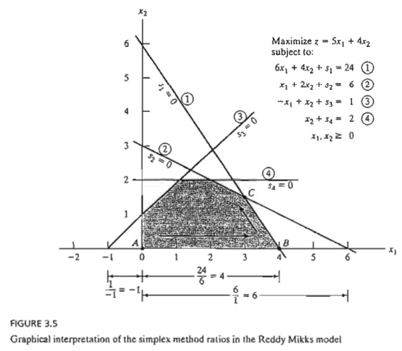
The minimum nonnegative ratio automatically identifies the current basic variable s1 as the leaving variable and assigns the entering variable x1 the new value of 4.
The new solution point B is determined by "swapping" the entering variable x1 and the leaving variable sl in the simplex tableau to produce the following sets of nonbasic and basic variables:
Nonbasic (zero) variables at B: (sI, x2)
Basic variables at B: (x1, s2, s3, s4)
The swapping process is based on the Gauss-Jordan row operations. It identifies the entering variable column as the pivot column and the leaving variable row as the pivot row. The intersection of the pivot column and the pivot row is called the pivot element. The following tableau is a restatement of the starting tableau with its pivot TOW and column highlighted.
The Gauss-Jordan computations needed to produce the new basic solution include two types.
a. Replace the leaving variable in the Basic column with the entering variable.
b. New pivot row = Current pivot row + Pivot element
2. All other rows, including z
New Row == (Current row) - (Its pivot column coefficient) X (New pivot row)
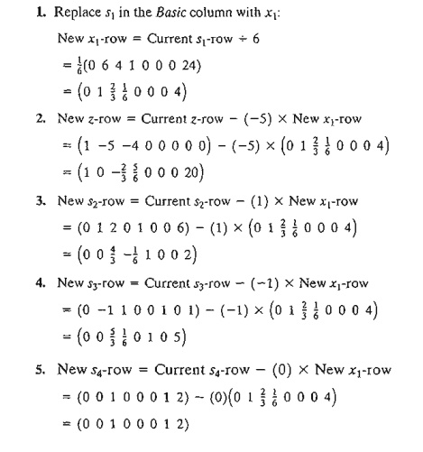
These computations are applied to the preceding tableau in the following manner:
1. Replace sl in the Basic column with xl:
New xl-row == Current sl-row + 6
The new basic solution is (x1, s2, s3, s4), and the new tableau becomes
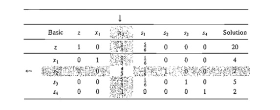
Observe that the new tableau has the same properties as the starting tableau. When we set the new nonbasic variables x2 and s1 to zero, the Solution column automatically yields the new basic solution (xl = 4, s2 = 2, s3 = 5, s4 = 2). This "conditioning" of the tableau is the result of the application of the Gauss-Jordan row operations. The corresponding new objective value is z = 20, which is consistent with
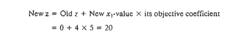
In the last tableau, the optimality condition shows that x2 is the entering variable. The feasibility condition produces the following
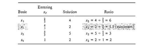
Thus, s2 leaves the basic solution and new value of x2 is 1.5. The corresponding increase in z is 2/3 * x2 = 2/3 * 1.5 = 1, which yields new z = 20 + 1 = 21.
Replacing s2 in the Basic column with entering x2, the following Gauss-Jordan row operations are applied:
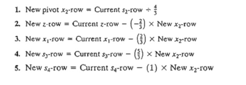
These computations produce the following tableau:
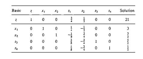
Based on the optimality condition, none of the z-row coefficients associated with the nonbasic variables, sl and s2, are negative. Hence, the last tableau is optimal.
The optimum solution can be read from the simplex tableau in the following manner. The optimal values of the variables in the Basic column are given in the right-hand-side Solution column and can be interpreted as
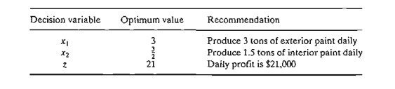
You can verify that the values s1 = s2 = 0, s3 = 5/2 , s4 =1/2 are consistent with the given values of xl and x2 by substituting out the values of x1 and x2 in the constraints.
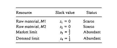
The solution also gives the status of the resources. A resource is designated as scarce if the activities (variables) of the model use the resource completely. Otherwise, the resource is abundant. This information is secured from the optimum tableau by checking the value of the slack variable associated with the constraint representing the resource. If the slack value is zero, the resource is used completely and, hence, is classified as scarce. Otherwise, a positive slack indicates that the resource is abundant. The following table classifies the constraints of the model:
Remarks. The simplex tableau offers a wealth of additional information that includes:
2. Post-optimal analysis, which deals with finding a new optimal solution when the data of .the model are changed.
Section 3.6 deals with sensitivity analysis. The more involved topic of post-optimal analysis is covered in Chapter 4.
TORA Moment.
The Gauss-Jordan computations are tedious, voluminous, and, above all, boring. Yet, they are the least important, because in practice these computations are carried out by the computer. What is important is that you understand how the simplex method works. TORA's interactive user-guided option (with instant feedback) can be of help in this regard because it allows you to decide the course of the computations in the simplex method without the burden of carrying out the Gauss-Jordan calculations. To use TORA with the Reddy Mikks problem, enter the model and then, from the SOLVEIMODIFY menu, select Solve ~ Algebraic => Iterations ~ Ail-SliiCk. (The All-Slack selection indicates that the starting basic solution consists of slack variables only. The remaining options will be presented in Sections 3.4,4.3, and 7.4.2.) Next, click : Go To Output Screen. You can generate one or all iterations by clicking Next Iteration: or All Iterations. If you opt to generate the iterations one at a time, you can interactively specify the entering and leaving variables by clicking the headings of their corresponding column and row. If your selections are correct, the column turns green and the row turns red. Else, an error message will be posted.
3. Summary of the Simplex Method
So far we have dealt with the maximization case. In minimization problems, the optimality condition calls for selecting the entering variable as the nonbasic variable with the most positive objective coefficient in the objective equation, the exact opposite rule of the maximization case. This follows because max z is equivalent to min (-z). As for the feasibility condition for selecting the leaving variable, the rule remains unchanged.
Optimality condition. The entering variable in a maximization (minimization) problem is the nonbasic variable having the most negative (positive) coefficient in the z-row. Ties are broken arbitrarily. The optimum is reached at the iteration where all the z-row coefficients of the nonbasic variables are nonnegative (nonpositive).
Feasibility condition. For both the maximization and the minimization problems, the leaving variable is the basic variable associated with the smallest nonnegative ratio (with strictly positive denominator). Ties are broken arbitrarily.
Gauss-Jordan row operations.
1. Pivot row
a. Replace the leaving variable in the Basic column with the entering variable.
b. New pivot row = Current pivot row -+- Pivot element
2. All other rows, including z
New row = (Current row) - (pivot column coefficient) X (New pivot row)
The steps of the simplex method are
Step 1. Determine a starting basic feasible solution.
Step 2. Select an entering variable using the optimality condition. Stop if there is no entering variable; the last solution is optimal. Else, go to step 3.
Step 3. Select a leaving variabLe using the feasibility condition.
Step 4. Determine the new basic solution by using the appropriate Gauss-Jordan computations. Go to step 2.
PROBLEM SET 3.3B
1. This problem is designed to reinforce your understanding of the simplex feasibility condition. In the first tableau in Example 3.3-1, we used the minimum (nonnegative) ratio test to determine the leaving variable. Such a condition guarantees that none of the new val-ues of the basic variables will become negative (as stipulated by the definition of the LP).
To demonstrate this point, force s2, instead of s1 to leave the basic solution. Now, look at the resulting simplex tableau, and you will note that 51 assumes a negative value (= -12), meaning that the new solution is infeasible. This situation will never occur if we employ the minimum-ratio feasibility condition.
2. Consider the following set of constraints:
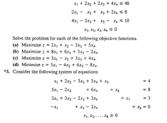
Let x5, x6,…., and xg be a given initial basic feasible solution. Suppose that x1 becomes basic. Which of the given basic variables must become nonbasic at zero level to guarantee that all the variables remain nonnegative, and what is the value of x1 in the new solution? Repeat this procedure for x2, x3, and x4.
a.Solve the problem by inspection (do not use the Gauss-Jordan row operations), and justify the answer in terms of the basic solutions of the simplex method.
b.Repeat (a) assuming that the objective function calls for minimizing z = x1.
5. Solve the following problem by inspection, and justify the method of solution in terms of the basic solutions of the simplex method.
(Hint: A basic solution consists of one variable only.)
4. The following tableau represents a specific simplex iteration. All variables are nonnegative. The tableau is not optimal for either a maximization or a minimization problem. Thus, when a nonbasic variable enters the solution it can either increase or decrease z or leave it unchanged, depending on the parameters of the entering nonbasic variable.
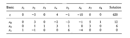
a. Categorize the variables as basic and nonbasic and provide the current values of all the variables.
*b. Assuming that the problem is of the maximization type, identify the nonbasic variables that have the potential to improve the value of z. If each such variable enters the basic solution, determine the associated leaving variable, if any, and the associated change in z. Do not use the Gauss-Jordan row operations.
c. Repeat part (b) assuming that the problem is of the minimization type.
d. Which nonbasic variable(s) will not cause a change in the value of z when selected to enter the solution?
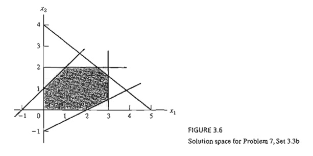
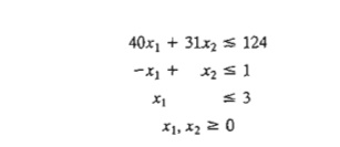
7. Consider the two-dimensional solution space in Figure 3.6.
a.Suppose that the objective function is given as
Maximize z = 3x1 + 6x2
If the simplex iterations start at point A, identify the path to the optimum point E.
b. Determine the entering variable, the corresponding ratios of the feasibility condition, and the change in the value of z, assuming that the starting iteration occurs at point A and that the objective function is given as
Maximize z = 4x1 + x2
(c) Repeat (b), assuming that the objective function is
Maximize z = xl + 4x2
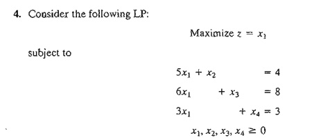
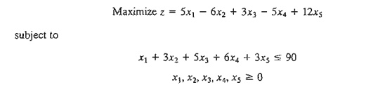
8. Consider the following LP:
Maximize z = 16xI + 15x2
subject to
a. Solve the problem by the simplex method, where the entering variable is the nonbasic variable with the most negative z-row coefficient.
b. Resolve the problem by the simplex algorithm, always selecting the entering variable as the nonbasic variable with the least negative z-row coefficient.
c. Compare the number of iterations in (a) and (b). Does the selection of the entering variable as the nonbasic variable with the most negative z-row coefficient lead to a smaller number of iterations? What conclusion can be made regarding the optimality condition?
d. Suppose that the sense of optimization is changed to minimization by multiplying z by -1. How does this change affect the simplex iterations?
*9. In Example 3.3-1, show how the second best optima) value of z can be determined from the optimal tableau.
10. Can you extend the procedure in Problem 9 to determine the third best optimal value. of z?
1L The Gutchi Company manufactures purses, shaving bags, and backpacks. The construction includes leather and synthetics, leather being the scarce raw material. The production process requires two types of skilled labor: sewing and finishing. The following table gives the availability of the resources, their usage by the three products, and the profits per unit.
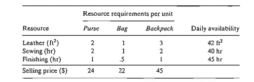
a. Formulate the problem as a linear program and find the optimum solution (using TORA, Excel Solver, or AMPL).
b. From the optimum solution determine the status of each resource.
12. TO RA experiment. Consider the following LP:
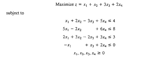
a. Use TORA's iterations option to determine the optimum tableau.
b. Select any nonbasic variable to "enter" the basic solution, and click Next Iteration to produce the associated iteration. How does the new objective value compare with the optimum in (a)? The idea is to show that the tableau in (a) is optimum because none of the nonbasic variables can improve the objective value.
13. TORA experiment. In Problem 12, use TORA to find the next-best optimal solution.
Related Topics