Chapter: Operations Research: An Introduction : The Simplex Method and Sensitivity Analysis
Special Cases in the Simplex Method
SPECIAL CASES IN THE SIMPLEX METHOD
This
section considers four special cases that arise in the use of the simplex
method.
1. Degeneracy
2. Alternative
optima
3. Unbounded
solutions
4. Nonexisting
(or infeasible) solutions
Our
interest in studying these special cases is twofold: (1) to present a theoretical explanation of these
situations and (2) to provide a practical
interpretation of what these special results could mean in a real-life problem.
1. Degeneracy
In the
application of the feasibility condition of the simplex method, a tie for the
mini-mum ratio may occur and can be broken arbitrarily. When this happens, at
least one basic variable will be zero
in the next iteration and the new solution is said to be degenerate.
There is
nothing alarming about a degenerate solution, with the exception of a small
theoretical inconvenience, called cycling or circling, which we shall discuss
short-ly. From the practical standpoint, the condition reveals that the model
has at least one redundant constraint.
To provide more insight into the practical and theoretical im-pacts of
degeneracy, a numeric example is used.
Example
3.5-1 (Degenerate
Optimal Solution)
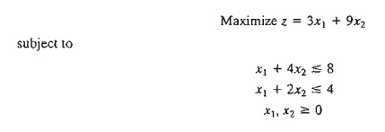
Given the
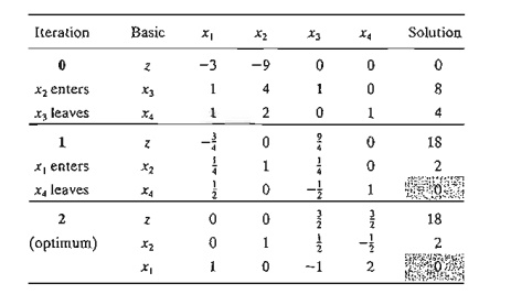
slack variables x3 and x4, the following tableaus
provide the simplex iterations of the problem:
In
iteration 0, x3 and x4 tie for the leaving variable,
leading to degeneracy in iteration 1 because the basic variable x4 assumes
a zero value. The optimum is reached in one additional iteration.
What is
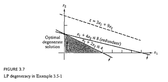
the practical implication of degeneracy? Look at the graphical solution in
Figure 3.7. Three lines pass through the optimum point (x1 = 0, x2
= 2). Because this is a two-dimensional problem, the point is overdetermined and one of the
constraints is redundant? In practice, the mere knowledge that some resources
are superfluous can be valuable during the implementa-tion of the solution. The
information may also lead to discovering irregularities in the construc-tion of
the model. Unfortunately, there are no efficient computational techniques for
identifying the redundant constraints directly from the tableau.
From the
theoretical standpoint, degeneracy has two implications. The first is the
phe-nomenon of cycling or circling. Looking at simplex iterations 1 and 2, you
will notice that the objective value does not improve (z = 18). It is thus possible for the simplex
method to enter a repetitive sequence of iterations, never improving the
objective value and never satisfying the optimality condition (see Problem 4,
Set 3.5a). Although there are methods for eliminat-ing cycling, these methods
lead to drastic slowdown in computations. For this reason, most LP codes do not
include provisions for cycling, relying on the fact that it is a rare
occurrence in practice.
The
second theoretical point arises in the examination of iterations 1 and 2. Both
iterations, though differing in the basic-nonbasic categorization of the
variables, yield identical values for all the variables and objective
value-namely,
x1=0,
x2= 2, x3= 0, x4=0, z=18
Is it
possible then to stop the computations at iteration 1 (when degeneracy first appears),
even though it is not optimum? The answer is no, because the solution may be temporarily de-generate as Problem 2,
Set 3.5a demonstrates.
PROBLEM SET 3.5A
*1.
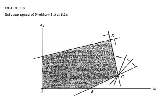
Consider the graphical solution space in Figure 3.8. Suppose that the simplex
iterations start at A and that the optimum solution
occurs at D. Further, assume that the objective function is defined such that at A, xI
enters the solution first.
a. Identify
(on the graph) the corner points that define the simplex method path to the
optimum point.
b. Determine
the maximum possible number of simplex iterations needed to reach the optimum
solution, assuming no cycling.
2. Consider
the following LP:
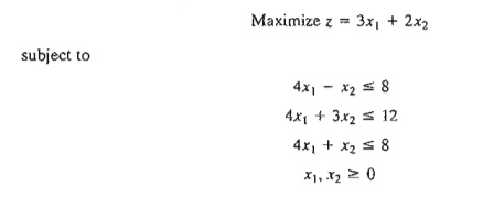
a. Show
that the associated simplex iterations are temporarily degenerate (you may use
TORA for convenience).
b. Verify
the result by solving the problem graphically (TORA's Graphic module can be
used here).
3. TORA experiment. Consider the LP in Problem 2.
a. Use
TORA to generate the simplex iterations. How many iterations are needed to
reach the optimum?
b. Interchange
constraints (1) and (3)
and re-solve the problem with TORA. How many iterations are needed to solve the
problem?
c. Explain
why the numbers of iterations in (a) and (b) are different.
4. TORA Experiment Consider
the following LP (authored by E.M. Beale to demonstrate cycling):
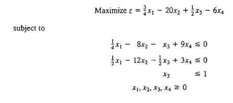
From
TORA's SOLVEIMODIFY menu, select Solve => Algebraic. => Iterations => All-slack. Next, "thumb" through
the successive simplex iterations using the command Next iteration (do not use All iterations,
because the simplex method will then cycle in-definitely). You will notice that
the starting all-slack basic feasible solution at iteration 0 will reappear
identically in iteration 6. This example illustrates the occurrence of cycling
in the simplex iterations and the possibility that the algorithm may never
converge to the optimum solution.
It is interesting that cycling will
not occur in this example if all the coefficients in this LP are converted to integer
values by using proper multiples (try it!).
2. Alternative Optima
When the
objective function is parallel to a nonredundant binding constraint (i.e., a constraint that is satisfied as an
equation at the optimal solution), the objective function can assume the same
optimal value at more than one solution point, thus giving rise to alternative
optima. The next example shows that there is an infinite number of such solutions. It also demonstrates the practical significance of encoun-tering such
solutions.
Example 3.5-2 (Infinite Number of Solutions)
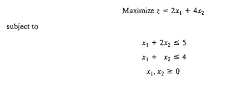
Figure
3.9 demonstrates how alternative optima can arise in the LP model when the
objec-tive function is parallel to a binding constraint. Any point on the line segment Be represents an alternative
optimum with the same objective value z
== 10.
The
iterations of the model are given by the following tableaus.
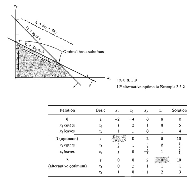
Iteration
1 gives the optimum solution x1 = 0, x2 = 5/2 and z = 10, which coincides
with point B in Figure 3.9. How do we know from this tableau that alternative optima
exist? Look at the z-equation coefficients of the nonbasic variables in iteration 1. The coefficient of nonbasic x1 is zero,
indicating that x1 can enter the basic solution
without changing the value of z, but causing a change in the values of the
variables. Iteration 2 does just that-letting x1 enter the basic solution and
forcing x4 to leave. The
new solution point occurs at C(xI = 3, x2 = 1, z = 10). (TORA's Iteratioris option allows determining one
alternative optimum at a time.)
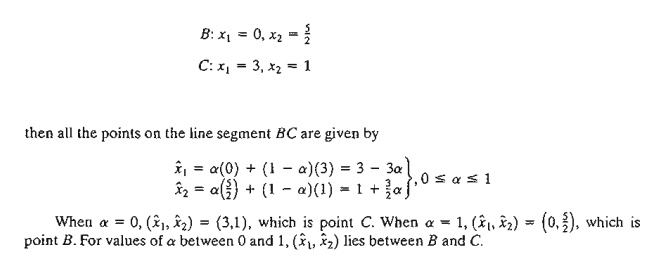
The
simplex method determines only the two corner points Band C. Mathematically, we can determine
all the points (x1, x2)
on the line segment Be as a nonnegative. weighted
average of points Band C. Thus, given
Remarks. In practice, alternative optima
are useful because we can choose from many solutions without experiencing
deterioration in the objective value. For instance, in the present ex-ample,
the solution at B shows that activity
2 only is at a positive level, whereas at C both activities are positive. If the example represents a
product-mix situation, there may be advan-tages in producing two products
rather than one to meet market competition. In this ease, the so-lution at C
may be more appealing.
PROBLEM
SeT 3.5B
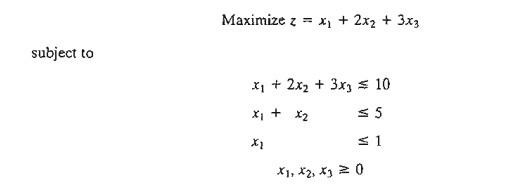
*1. For
the following LP, identify three alternative optimal basic solutions, and then
write a general expression for all the nonbasic alternative optima comprising
these three basic solutions.
Note: Although the problem has more
than three alternative basic solution optima, you are only required to identify three of them. You may use TORA
for convenience.
2. Solve
the following LP:

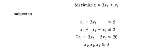
From the
optimal tableau, show that all the alternative optima are not corner points
(i.e., nonbasic). Give a two-dimensional graphical demonstration of the type of
solu-tion space and objective function that will produce this result. (You may
use TORA for convenience.)
3. For
the following LP, show that the optimal solution is degenerate and that none of
the alternative solutions are corner points (you may use TORA for convenience).
3. Unbounded Solution
In some
LP models, the values of the variables may be increased indefinitely without
violating any of the constraints-meaning that the solution space is unbounded in at least one variable. As a
result, the objective value may increase (maximization case) or decrease
(minimization case) indefinitely. In this case, both the solution space and the
optimum objective value are unbounded.
Unboundedness
points to the possibility that the model is poorly constructed. The most likely
irregularity in such models is that one or more nonredundant constraints have
not been accounted for, and the parameters (constants) of some constraints may
not have been estimated correctly.
The
following examples show how unboundedness, in both the solution space and the
objective value, can be recognized in the simplex tableau.
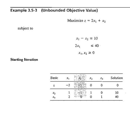
In the
starting tableau, both xl and x2 have negative z-equation
coefficients. Hence either one can improve the solution. Because xl
has the most negative coefficient, it is normally selected as the entering
variable. However, all the constraint coefficients under x2 (Le.,
the denominators of the ratios of the feasibility condition) are negative or
zero. This means that there is no leaving variable and that x2 can
be increased indefinitely without violating any of the constraints (compare
with the graphical interpretation of the minimum ratio in Figure 3.5). Because
each unit increase in xl will increase z by 1, an infinite increase
in x2 leads to an infinite increase in z.
Thus, the
problem has no bounded solution. This result can be seen in Figure 3.10. The
solution space is unbounded in the direction of x2, and the value of
z can be increased indefinitely. Remarks.
What would have happened if we had applied the strict optimality condition that
3.5 calls for xl to enter the solution? The answer is that a
succeeding tableau would eventually have led to an entering variable with the
same characteristics as x2. See Problem 1, Set3.5c.
PROBLEM SET 3.5C
1. TORA
Experiment. Solve Example 3.5-3 using TORA's Iterations option and show that
even though the solution starts with xl as the entering variable
(per the optimality condition), the simplex algorithm will point eventually to
an unbounded solution.
*2.
Consider the LP:
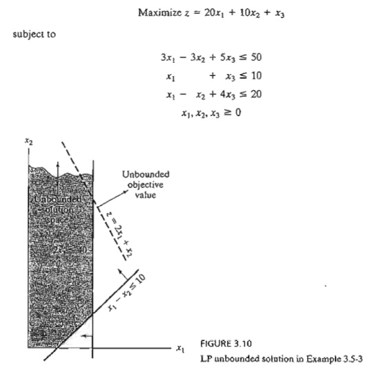
a. By
inspecting the constraints, determine the direction (xI. x2, or x3) in which the solution space is unbounded.
b. Without
further computations, what can you conclude regarding the optimum objective
value?
3. In
some ill-constructed LP models, the solution space may be unbounded even though
the problem may have a bounded objective value. Such an occurrence can point
only to irregularities in the construction of the model. In large problems, it
may be difficult to detect unboundedness by inspection. Devise a procedure for
determining whether or not a solution space is unbounded.
4. Infeasible Solution
LP models
with inconsistent constraints have no feasible solution. This situation can never
occur if all the constraints are of
the type ≤ with
nonnegative right-hand sides because the slacks provide a feasible solution.
For other types of constraints, we use artificial variables. Although the
artificial variables are penalized in the objective function to force them to
zero at the optimum, this can occur only if the model has a feasible space.
Otherwise, at least one artificial variable will be positive in the optimum iteration. From the practical standpoint,
an infeasible space points to the possibility that the model is not formulated
correctly.
Example 3.5-4 (Infeasible
Solution Space)
Consider
the following LP:
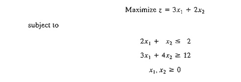
Using the
penalty M = 100 for the artificial variable R, the following tableaux provide
the simplex iterations of the model.

Optimum
iteration 1 shows that the artificial variable R is positive (= 4),
which indicates that the problem is infeasible. Figure 3.11 demonstrates the
infeasible solution space. By allowing
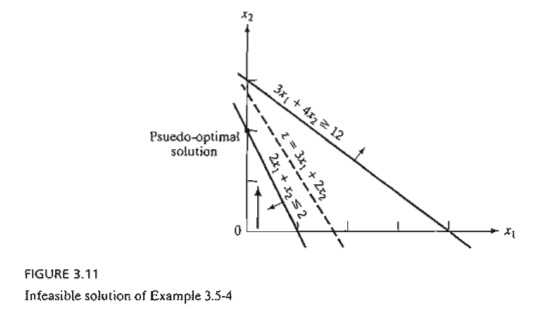
the
artificial variable to be positive, the simplex method, in essence, has
reversed the direction of the inequality from 3x1 + 4x2 ≥ 0: 12 to 3xl + 4x2 ≤12 (can you explain how?). The
result is what we may call a pseudo-optimal
solution.
PROBLEM
SET 3.50
*1.
Tooleo produces three types of tools, T1, T2,
and T3. The tools use two raw materials, M1
and M2, according to the data in the following table:

The
available daily quantities of raw materials M1
and M2 are 1000 units and 1200 units,
respectively. The marketing department informed the production manager that
according to their research, the daily demand for all three tools must be at
least 500 units. Will the manufacturing department be able to satisfy the
demand? If not, what is the most Toolco can
provide of the three tools?
2. TO RA Experiment. Consider
the LP model
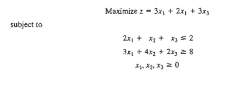
Use
TORA's Iterations => M-Meth6d to show that the optimal
solution includes an artificial basic variable, but at zero level. Does the
problem have a feasible optimal
solution?
Related Topics