Artificial Starting Solution: M-Method and Two-Phase Method

ARTIFICIAL STARTING SOLUTION

As demonstrated in Example 3.3-1, LPs in which all the constraints are (≤) with non-negative right-hand sides offer a convenient all-slack starting basic feasible solution. Models involving (=) and/or (≥) constraints do not.

The procedure for starting "ill-behaved" LPs with (=) and (≥) constraints is to use artificial variables that play the role of slacks at the first iteration, and then dispose of them legitimately at a later iteration. Two closely related methods are introduced here: the M-method and the two-phase method.

1. M-Method

The M-method starts with the LP in equation form (Section 3.1). If equation i does not have a slack (or a variable that can play the role of a slack), an artificial variable, R_i , is added to form a starting solution similar to the convenient all-slack basic solution. However, because the artificial variables are not part of the original LP model, they are assigned a very high penalty in the objective function, thus forcing them (eventually) to equal zero in the optimum solution. This will always be the case if the problem has a feasible solution. The following rule shows how the penalty is assigned in the cases of maximization and minimization:

Penalty Rule for Artificial Variables.

Given M, a sufficiently large positive value (mathematically, M -> ¥ ), the objec-tive coefficient of an artificial variable represents an appropriate penalty if:

Example3.4-1

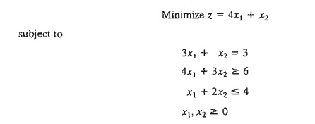
Using x₃ as a surplus in the second constraint and x₄ as a slack in the third constraint, the equation form of the problem is given as

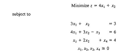
The third equation has its slack variable, x₄, but the first and second equations do not. Thus, we add the artificial variables R₁ and R₂ in the first two equations and penalize them in the objective function with M R₁ + M R₂ (because we are minimizing). The resulting LP is given as

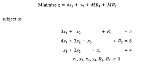
The associated starting basic solution is now given by (R₁, R₂, x₄ )  = (3,6,4).

From the standpoint of solving the problem on the computer, M must assume a numeric value. Yet, in practically all textbooks, including the first seven editions of this book, M is manipulated algebraically in all the simplex tableaus. The result is an added, and unnecessary, layer of difficulty which can be avoided simply by substituting an appropriate numeric value for M (which is what we do anyway when we use the computer). In this edition, we will break away from the long tradition of manipulating M algebraically and use a numerical substitution in-stead. The intent, of course, is to simplify the presentation without losing substance.

What value of M should we use? The answer depends on the data of the original LP. Recall that M must be sufficiently large relative to the original objective coefficients so it will act as a penalty that forces the artificial variables to zero level in the optimal solution. At the same time, since computers are the main tool for solving LPs, we do not want M to be too large (even though mathematically it should tend to infinity) because potential severe round-off error can result when very large values are manipulated with much smaller values. In the present example, the objective coefficients of x_l and x₂ are 4 and 1, respectively. It thus ap-pears reasonable to set M = 100.

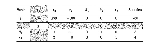
Using M = 100, the starting simplex tableau is given as follows (for convenience, the z-column is eliminated because it does not change in all the iterations):

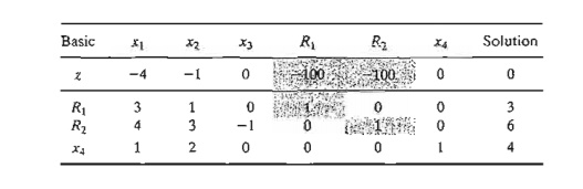
Before proceeding with the simplex method computations, we need to make the z-row consistent with the rest of the tableau. Specifically, in the tableau, x_l = x₂ = x₃ = 0, which yields the starting basic solution R₁ = 3, R₂ = 6_, and x₄ = 4. This solution yields z = 100 X 3 + 100 X 6 = 900 (instead of 0, as the right-hand side of the z-row currently shows). This inconsistency stems from the fact that R₁ and R₂ have nonzero coefficients (-100, -100) in the z-row (compare with the all-slack starting solution in Example 3.3-1, where the z-row coefficients of the slacks are zero).

We can eliminate this inconsistency by substituting out R₁ and R₂ in the z-row using the appropriate constraint equations. In particular, notice the highlighted elements (= 1) in the R1-row and the Rrrow. Multiplying each of R₁-row and R₂-row by 100 and adding the sum to the z-row will substitute out R₁ and R ₂ in the objective row-that is,

New z-row = Old z-row + (100 X  R₁-row + 100 X  R₂-row)

The modified tableau thus becomes (verify!)

Notice that z = 900, which is consistent now with the values of the starting basic feasible solu-tion: R_I = 3, R₂ = 6, and x₄ = 4.

The last tableau is ready for us to apply the simplex method using the simplex optimality and the feasibility conditions, exactly as we did in Section 3.3.2. Because we are minimizing the objective function, the variable Xl having the most positive coefficient in the z-row (= 696) en-ters the solution. The minimum ratio of the feasibility condition specifies R 1 as the leaving vari-able (verify!).

Once the entering and the leaving variables have been determined, the new tableau can be computed by using the familiar Gauss-Jordan operations.

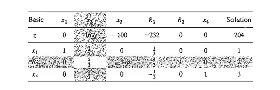
The last tableau shows that x₂ and R₂ are the entering and leaving variables, respectively.

Continuing with the simplex computations, two more iterations are needed to reach the optimum

Note that the artificial variables R₁ and R₂ leave the basic solution in the first and second iterations, a result that is consistent with the concept of penalizing them in the objective function.

Remarks. The use of the penalty M will not force an artificial variable to zero level in the final simplex iteration if the LP does not have a feasible solution (i.e., the constraints are not consistent). In this case, the final simplex iteration will include at least one artificial variable at a positive level. Section 3.5.4 explains this situation.

PROBLEM SET 3.4A

1. Use hand computations to complete the simplex iteration of Example 3.4-1 and obtain the optimum solution.

2. TORA experiment. Generate the simplex iterations of Example 3.4-1 using TORA's .iterations => M-fuethbd module (file toraEx3.4-l.txt). Compare the effect of using M = 1, M == 10, and M = 1000 on the solution. What conclusion can be drawn from this experiment?

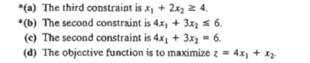
3. In Example 3.4-1, identify the starting tableau for each of the following (independent) cases, and develop the associated z-row after substituting out all the artificial variables:

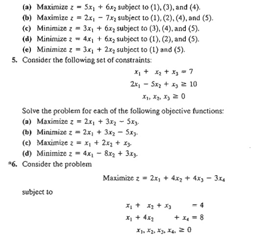
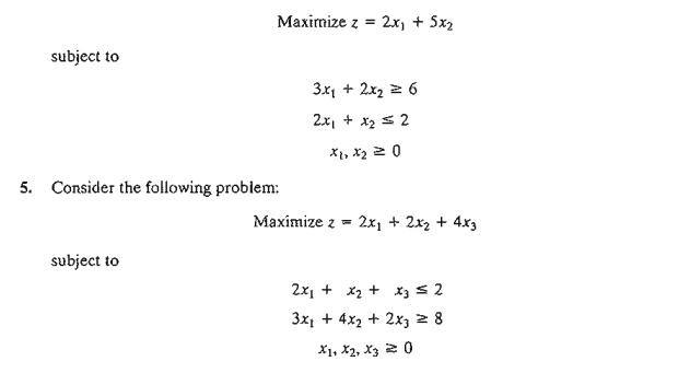
4. Consider the following set of constraints:

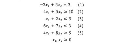
For each of the following problems, develop the z-row after substituting out the artificial variables:

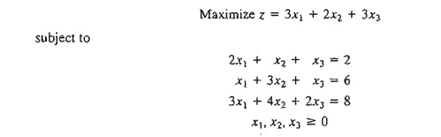
The problem shows that x₃ and x₄ can play the role of slacks for the two equations. They differ from slacks in that they have nonzero coefficients in the objective function. We can use x₃ and x₄ as starting variable, but, as in the case of artificial variables, they must be substituted out in the objective function before the simplex iterations are carried out. Solve the problem with x₃ and x₄ as the starting basic variables and without using any artificial variables.

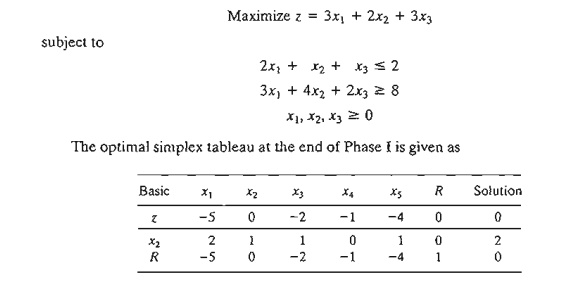
7. Solve the following problem using x₃ and x₄ as starting basic feasible variables. As in Problem 6, do not use any artificial variables.

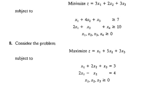
The variable x₃ plays the role of a slack. Thus, no artificial variable is needed in the first constraint. However, in the second constraint, an artificial variable is needed. Use this starting solution (i.e., x₃ in the first constraint and R₂ in the second constraint) to solve this problem.

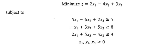
9. Show how the M-method will indicate that the following problem has no feasible solution.

2. Two-Phase Method

In the M-method, the use of the penalty M, which by definition must be large relative . to the actual objective coefficients of the model, can result in roundoff error that may impair the accuracy of the simplex calculations. The two-phase method alleviates this difficulty by eliminating the constant M altogether. As the name suggests, the method solves the LP in two phases: Phase I attempts to find a starting basic feasible solution, and, if one is found, Phase II is invoked to solve the original problem.

Summary of the Two-Phase Method

Phase I. Put the problem in equation form, and add the necessary artificial variables to the constraints (exactly as in the M-method) to secure a starting basic solution. Next, find a basic solution of the resulting equations that, regardless of whether the LP is maximization or minimization, always minimizes the sum of the artificial variables. If the minimum value of the sum is positive, the LP problem has no feasible solution, which ends the process (recall that a positive artificial variable signifies that an original constraint is not satisfied). Otherwise, proceed to Phase II.

Phase II. Use the feasible solution from Phase I as a starting basic feasible solu-tion for the original problem.

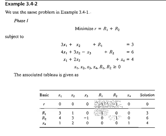
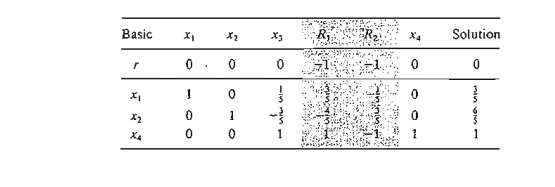
As in the M-method, R₁ and R₂ are substituted out in the r-row by using the following computations:

New r-row = Old r-row + (1 X  R,-row + 1 x R-row)

The new r-row is used to solve Phase I of the problem, which yields the following optimum tableau (verify with TORA's Iterations => Two-phase Method):

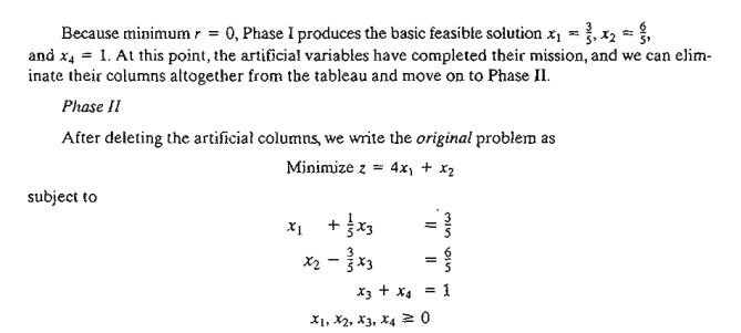
Essentially, Phase I is a procedure that transforms the original constraint equations in a manner that provides a starting basic feasible solution for the problem, if one exists. The tableau associated with Phase II problem is thus given as

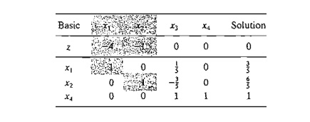
Again, because the basic variables x₁ and x₂ have nonzero coefficients in the z-row, they must be substituted out, using the following computations.

New z-row = Old z-row + (4 X  x₁-row + 1 X x₂-row)

The initial tableau of Phase II is thus given as

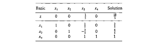
Because we are minimizing, x₃ must enter the solution. Application of the simplex method will produce the optimum in one iteration (verify with TORA).

Remarks. Practically all commercial packages use the two-phase method to solve LP. The M-method with its potential adverse roundoff error is probably never used in practice. Its inclusion in this text is purely for historical reasons, because its development predates the development of the two-phase method.

The removal of the artificial variables and their columns at the end of Phase I can take place only when they are all nonbasic (as Example 3.4-2 illustrates). If one or more artificial variables are basic (at zero level) at the end of Phase I, then the following additional steps must be under-taken to remove them prior to the start of Phase II.

Step 1. Select a zero artificial variable to leave the basic solution and designate its row as the pivot row. The entering variable can be any nonbasic (nonartificiaI) variable with a nonzero (positive or negative) coefficient in the pivot row. Perform the associated simplex iteration.

Step 2. Remove the column of the (just-leaving) artificial variable from the tableau. If all the zero artificial variables have been removed, go to Phase II. Otherwise, go back to Step 1.

The logic behind Step 1 is that the feasibility of the remaining basic variables will not be affected when a zero artificial variable is made nonbasic regardless of whether the pivot element is positive or negative. Problems 5 and 6, Set 3Ab illustrate this situation. Problem 7 provides an additional detail about Phase I calculations.

PROBLEM SET 3.4B

*1.  In Phase I, if the LP is of the maximization type, explain why we do not maximize the sum of the artificial variables in Phase I.

2. For each case in Problem 4, Set 3.4a, write the corresponding Phase I objective function.

3. Solve Problem 5, Set 3.4a, by the two-phase method.

4. Write Phase I for the following problem, and then solve (with TORA for convenience) to show that the problem has no feasible solution.

a. Show that Phase I will terminate with an artificial basic variable at zero level (you may use TORA for convenience).

b. Remove the zero artificial variable prior to the start of Phase II, then carry out Phase II iterations.

6. Consider the following problem:

a. Show that Phase I terminates with two zero artificial variables in the basic solution (useTORA for convenience).

b. Show that when the procedure of Problem 5(b) is applied at the end of Phase I, only one of the two zero artificial variables can be made nonbasic.

c. Show that the original constraint associated with the zero artificial variable that can-not be made nonbasic in (b) must be redundant-hence, its row and its column can be dropped altogether at the start of Phase II.

*7. Consider the following LP:

Explain why the nonbasic variables x₁, x₃, x₄, and x_s can never assume positive values at the end of Phase II. Hence, conclude that their columns can dropped before we start Phase II. In essence, the removal of these variables reduces the constraint equations of the problem to x₂ = 2. This means that it will not be necessary to carry out Phase II at all, because the solution space is reduced to one point only.

8. Consider the LP model

Show how the inequalities can be modified to a set of equations that requires the use of a single artificial variable only (instead of two).