Chapter: Compilers : Principles, Techniques, & Tools : Lexical Analysis
Recognition of Tokens
Recognition of Tokens
1 Transition Diagrams
2 Recognition of Reserved Words
and Identifiers
3 Completion of the Running
Example
4 Architecture of a
Transition-Diagram-Based Lexical Analyzer
5 Exercises for Section 3.4
In the previous section we learned how to express patterns using regular
expres-sions. Now, we must study how to take the patterns for all the needed
tokens and build a piece of code that examines the input string and finds a
prefix that is a lexeme matching one of the patterns. Our discussion will make
use of the following running example.
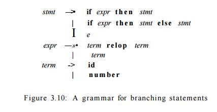
Example 3.8 : The grammar fragment of Fig. 3.10 describes a simple form of branching
statements and conditional expressions. This syntax is similar to that of the
language Pascal, in that t h e n appears explicitly after conditions.
For relop, we use the
comparison operators of languages like Pascal or SQL, where = is
"equals" and <> is "not equals," because it presents
an interesting structure of lexemes.
The terminals of the grammar, which are if, then, else, relop, id, and number,
are the names of tokens as far as the lexical analyzer is concerned. The patterns for these tokens are
described using regular definitions, as in Fig. 3.11. The patterns for id and number are similar to what we saw in Example 3.7.

For this language, the lexical analyzer will recognize the keywords if,
then, and e l s e , as well as lexemes that match the patterns for relop, id,
and number. To simplify matters, we make the common assumption that keywords
are also reserved words: that is, they are not identifiers, even though their
lexemes match the pattern for identifiers.
In addition, we assign the lexical analyzer the job of stripping out
white-space, by recognizing the "token" ws defined by:
ws -» ( blank | tab j newline )+
Here, blank, tab, and newline are abstract symbols that we
use to express the ASCII characters of the same names. Token ws is different from the other tokens in
that, when we recognize it, we do not return it to the parser, but rather
restart the lexical analysis from the character that follows the whitespace. It
is the following token that gets returned to the parser.
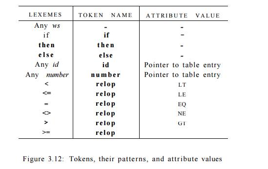
Our goal for the lexical analyzer is summarized in Fig. 3.12. That table
shows, for each lexeme or family of lexemes, which token name is returned to
the parser and what attribute value, as discussed in Section 3.1.3, is
returned. Note that for the six relational operators, symbolic constants LT, LE, and so on are used as the
attribute value, in order to indicate which instance of the token relop we have found. The particular
operator found will influence the code that is output from the compiler. •
1. Transition Diagrams
As an intermediate step in the construction of a lexical analyzer, we
first convert patterns into stylized flowcharts, called "transition
diagrams." In this section, we perform the conversion from
regular-expression patterns to transition dia-grams by hand, but in Section
3.6, we shall see that there is a mechanical way to construct these diagrams
from collections of regular expressions.
Transition diagrams have a collection of nodes or circles, called states. Each state
represents a condition that could occur during the process of scanning the
input looking for a lexeme that matches one of several patterns. We may think
of a state as summarizing all we need to know about what characters we have seen
between the lexemeBegin pointer and the forward pointer (as in the situation of
Fig. 3.3).
Edges are directed from one state of the transition diagram to another.
Each edge is labeled by a symbol or set of symbols. If we are in some
state 5, and the next input symbol is a, we look for an edge out of state s
labeled by a (and perhaps by other symbols, as well). If we find such an edge,
we advance the forward pointer arid enter the state of the transition diagram
to which that edge leads. We shall assume that all our transition diagrams are
deterministic, meaning that there is never more than one edge out of a given
state with a given symbol among its labels. Starting in Section 3.5, we shall
relax the condition of determinism, making life much easier for the designer of
a lexical analyzer, although trickier for the implementer. Some important
conventions about transition diagrams are:
1. Certain states are said to be accepting, or final. These states
indicate that a lexeme has been found, although the actual lexeme may not
consist of all positions between the lexemeBegin and forward pointers. We
always indicate an accepting state by a double circle, and if there is an
action to be taken — typically returning a token and an attribute value to the
parser — we shall attach that action to the accepting state.
2. In addition, if it is necessary to retract the forward pointer one
position (i.e., the lexeme does not include the symbol that got us to the
accepting state), then we shall additionally place a * near that accepting
state. In our example, it is never necessary to retract forward by more than
one position, but if it were, we could attach any number of *'s to the
accepting state.
3. One state is designated the start state, or initial state; it is
indicated by an edge, labeled "start," entering from nowhere. The
transition diagram always begins in the start state before any input symbols
have been read.
Example 3 . 9 : Figure 3.13 is a transition diagram that recognizes the lexemes matching the token relop. We begin in state 0, the start
state. If we see < as the first input symbol, then among the lexemes that
match the pattern for relop we can
only be looking at <, <>, or <=. We therefore go to state 1, and
look at the next character. If it is =, then we recognize lexeme <=, enter
state 2, and return the token relop
with attribute LE, the symbolic constant representing this particular
comparison operator. If in state 1 the next character is >, then instead we
have lexeme <>, and enter state 3 to return an indication that the
not-equals operator has been found. On any other character, the lexeme is <,
and we enter state 4 to return that information. Note, however, that state 4
has a * to indicate that we must retract the input one position.
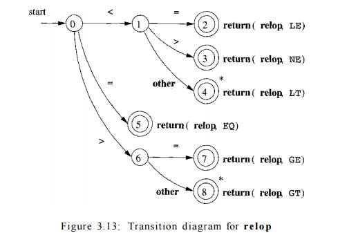
On the other hand, if in state 0 the first character we see is =, then
this one character must be the lexeme. We immediately return that fact from
state 5.
The remaining possibility is that the first character is >. Then, we
must enter state 6 and decide, on the basis of the next character, whether the
lexeme is >= (if we next see the = sign), or just > (on any other character). Note that if, in state 0, we see any
character besides <, =, or >,
we can not possibly be seeing a relop lexeme, so this transition diagram will
not be used.
2. Recognition of Reserved Words
and Identifiers
Recognizing keywords and identifiers presents a problem. Usually,
keywords like if or then are
reserved (as they are in our running example), so they are not identifiers even
though they look like identifiers.
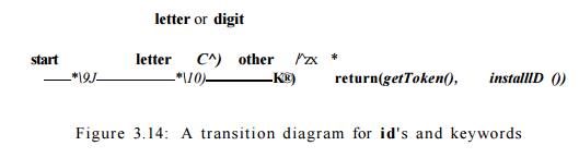
Thus, although we typically use a transition diagram like that of Fig. 3.14 to
search for identifier lexemes, this diagram will also recognize the keywords
if, then, and e l s e of our running example.
There are two ways that we can handle reserved words that look like
identifiers:
Install the reserved words in the
symbol table initially. A field of the symbol-table entry indicates that these
strings are never ordinary identi- fiers, and tells which token they represent.
We have supposed that this method is in use in Fig. 3.14. When we find an
identifier, a call to installlD
places it in the symbol table if it is not already there and returns a pointer
to the symbol-table entry for the lexeme found. Of course, any identifier not
in the symbol table during lexical analysis cannot be a reserved word, so its
token is id. The function getToken examines the symbol table entry
for the lexeme found, and returns whatever token name the symbol table says
this lexeme represents — either id
or one of the keyword tokens that was initially installed in the table.
1.
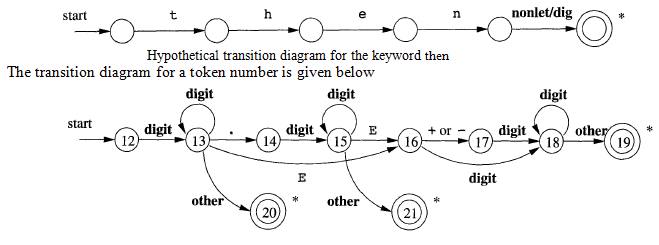
Create separate transition
diagrams for each keyword; an example for the keyword then is shown in Fig. 3.15. Note that such a transition diagram
consists of states representing the situation after each successive letter of
the keyword is seen, followed by a test for a "nonletter-or-digit,"
i.e., any character that cannot be the continuation of an identifier. It is
necessary to check that the identifier has ended, or else we would return token
then in situations where the correct token was id, with a lexeme like then e x
t value that has then as a proper prefix. If we adopt this approach, then we
must prioritize the tokens so that the reserved-word tokens are recognized in
preference to id, when the lexeme matches both patterns. We do not use this approach in our example,
which is why the states in Fig. 3.15 are unnumbered.
3. Completion of the Running
Example
The transition diagram for id's that we saw in Fig. 3.14 has a simple
structure. Starting in state 9, it checks that the lexeme begins with a letter
and goes to state 10 if so. We stay in state 10 as long as the input contains
letters and digits. When we first encounter anything but a letter or digit, we
go to state 11 and accept the lexeme found. Since the last character is not
part of the identifier, we must retract the input one position, and as
discussed in Section 3.4.2, we enter what we have found in the symbol table and
determine whether we have a keyword or a true identifier.
The transition diagram for token n u m b e r is shown in Fig. 3.16, and
is so far the most complex diagram we have seen. Beginning in state 12, if we
see a digit, we go to state 13. In that state, we can read any number of
additional digits. However, if we see anything but a digit or a dot, we have
seen a number in the form of an integer; 123 is an example. That case is
handled by entering state 20, where we return token n u m b e r and a pointer
to a table of constants where the found lexeme is entered. These mechanics are
not shown on the diagram but are analogous to the way we handled identifiers.
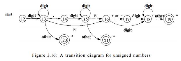
If we instead see a dot in state 13, then we have an "optional
fraction." State 14 is entered, and we look for one or more additional
digits; state 15 is used for that purpose. If we see an E, then we
have an "optional exponent," whose recognition is the job of states
16 through 19. Should we, in state 15, instead see anything but E or a
digit, then we have come to the end of the fraction, there is no exponent, and
we return the lexeme found, via state 21.
The final transition diagram, shown in Fig. 3.17, is for whitespace. In
that diagram, we look for one or more "whitespace" characters,
represented by delim in that diagram
— typically these characters would be blank, tab, newline, and perhaps other
characters that are not considered by the language design to be part of any
token.
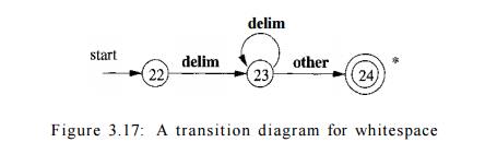
Note that in state 24, we have found a block of consecutive whitespace
characters, followed by a nonwhitespace character. We retract the input to
begin at the nonwhitespace, but we do not return to the parser. Rather, we must
restart the process of lexical analysis after the whitespace.
4. Architecture of a
Transition-Diagram-Based Lexical
Analyzer
There are several ways that a collection of transition diagrams can be
used to build a lexical analyzer. Regardless of the overall strategy, each
state is represented by a piece of code. We may imagine a variable s t a t e
holding the number of the current state for a transition diagram. A switch
based on the value of state takes us to
code for each of the possible states, where we find the action of that state. Often, the code for a state is itself a
switch statement or multiway branch that determines the next state by reading
and examining the next input character.
E x a m p l e 3 . 1 0 : In Fig. 3.18 we see a sketch of g e t R e l o p O , a C + + function whose job is to simulate the transition
diagram of Fig. 3.13 and return an object of type TOKEN, that is, a pair
consisting of the token name (which must be relop in this case) and an attribute value (the code for one of the
six comparison operators in this case). g e t R e l o p O first creates a new
object r e t Token and initializes its first component to RELOP, the symbolic
code for token relop.
We see the typical behavior of a state in case 0, the case where the
current state is 0. A function n e x t C h a r ( ) obtains the next character
from the input and assigns it to local variable c. We then check c for the
three characters we expect to find, making the state transition dictated by the
transition diagram of Fig. 3.13 in each case.
For example, if the next input character is =, we go to state 5.
If the next input character is not one that can begin a comparison
operator, then a function f a i l () is called. What f a i l () does depends on
the global error-recovery strategy of the lexical analyzer. It should reset the
forward pointer to lexemeBegin, in order to allow another transition diagram to
be applied to
TOKEN getRelopO
{
TOKEN retToken =
new(RELOP);
while(1) {
/* repeat character processing until a return
or failure occurs */
switch(state) {
case 0: c = nextCharQ;
if ( c == '<»
) state = 1;
else if ( c == '=' ) state = 5; else if ( c == '>' ) state - 6;
else fail(); /* lexeme is not a relop */ break;
case 1: ...
case 8: retract(); retToken.attribute = GT; return(retToken);
Figure 3.18: Sketch of implementation of relop transition diagram
the true beginning of the unprocessed input. It might then change the
value of state to be the start state for another transition diagram, which will search
for another token. Alternatively, if there is no other transition diagram that
remains unused, fail() could initiate an error-correction phase that will try to repair the
input and find a lexeme, as discussed in Section 3.1.4.
We also show the action for state 8 in Fig. 3.18. Because
state 8 bears a *, we must retract the input pointer one position (i.e., put c
back on the input stream). That task is accomplished by the function retract ( ) .
Since state 8 represents the recognition of lexeme >=, we set the second component
of the returned object, which we suppose is named attribute, to GT,
the code for this operator. •
To place the simulation of one transition diagram in perspective, let us
consider the ways code like Fig. 3.18 could fit into the entire lexical analyzer.
1.
We could arrange for the transition
diagrams for each token to be tried se-quentially. Then, the function f ail() of
Example 3.10 resets the pointer forward
and starts the next transition diagram, each time
it is called.
This method allows us to use transition diagrams
for the individual key-words, like the one suggested in Fig. 3.15. We have
oniy to use these before we use the diagram for id, in order for the keywords
to be reserved words.
We could run the various transition diagrams "in parallel,"
feeding the next input character to all of them and allowing each one to make
whatever transitions it required. If we use this strategy, we must be careful
to resolve the case where one diagram finds a lexeme that matches its pattern,
while one or more other diagrams are still able to process input. The normal
strategy is to take the longest prefix of the input that matches any pattern.
That rule allows us to prefer identifier the next to keyword then, or the
operator -> to -, for example.
The preferred approach, and the one we shall take up in the following
sections, is to combine all the transition diagrams into one. We allow the
transition diagram to read input until there is no possible next state, and
then take the longest lexeme that matched any pattern, as we discussed in item
(2) above. In our running example, this combination is easy, because no two
tokens can start with the same character; i.e., the first character immediately
tells us which token we are looking for. Thus, we could simply combine states
0, 9, 12, and 22 into one start state, leaving other transitions intact.
However, in general, the problem of combining transition diagrams for several
tokens is more complex, as we shall see shortly.
Exercises for Section 3.4
Exercise 3.4.1 : Provide transition diagrams to recognize the same
languages as each of the regular expressions in Exercise 3.3.2.
Exercise 3.4.2 : Provide transition diagrams to recognize the same
languages as each of the regular expressions in Exercise 3.3.5.
The following exercises, up to Exercise 3.4.12, introduce the
Aho-Corasick algorithm for recognizing a collection of keywords in a text
string in time proportional to the length of the text and the sum of the length
of the keywords.
This algorithm uses a special form of transition diagram called a trie.
A trie is a tree-structured transition diagram with distinct labels on the
edges leading from a node to its children. Leaves of the trie represent
recognized keywords.
Knuth, Morris, and Pratt presented an algorithm for recognizing a single
keyword &i&2 • • • K in a text string.
Here the trie is a transition diagram with n
states, 0 through n. State 0 is
the initial state, and state n represents
ac-ceptance, that is, discovery of the keyword. From each state s from 0 through n - 1, there is a
transition to state s + 1, labeled by
symbol ba+i. For example, the trie for the keyword ababaa is:
In order to process text strings rapidly and search those strings for a
key-word, it is useful to define, for keyword &i&2 • • •
&n and position s in that keyword
(corresponding to state s of its
trie), a failure function, f(s),
computed as in Fig. 3.19. The objective is that &i&2- " •&/(*) l s the
longest proper prefix of &1&2 • • • bs that is
also a suffix of
b1b2 • • •
bs. The reason
f(s) is important is that if we are trying to match a text
string for 61&2
• • • bn, and we have matched the first s
positions, but we then fail (i.e., the next position of the text string does
not hold bs+i), then f(s) is the longest
prefix of &1&2
• * • bn that could possibly match the text string up to the point we are at. Of
course, the next character of the text string must be &/(s )+i, or
else we still have problems and must consider a yet shorter prefix, which will
be &/(/(s )).
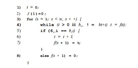
Figure 3.19: Algorithm to compute the failure function for keyword 6162 • • • bn
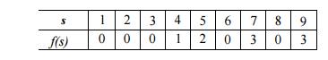
As an example, the failure function for the trie constructed above for ababaa is:

For instance, states 3 and 1 represent prefixes aba and a, respectively. /(3)
= 1 because a is the
longest proper prefix of aba that is also a suffix of aba. Also, /(2) =
0, because the longest proper
prefix of ab that is also a suffix is the empty string.
Exercise 3.4.3: Construct the failure function for the
strings:
abababaab.
aaaaaa.
abbaabb.
Exercise 3.4.4: Prove, by
induction on s, that the algorithm of Fig. 3.19 correctly
computes the failure function.
!! Exercise 3.4.5: Show that the assignment
t = f{t) in line (4) of Fig. 3.19 is executed
at most n times. Show that therefore,
the entire algorithm takes only 0(n) time
on a keyword of length n.
Having
computed the failure function for a keyword bib2 • • • bn, we can scan a string
a1a2---am in time 0(m) to tell whether the keyword occurs in the string. The
algorithm, shown in Fig. 3.20, slides the keyword along the string, trying to
make progress by matching the next character of the keyword with the next
character of the string. If it cannot do so after matching
s characters, then it
"slides" the keyword right s —
f(s) positions, so only the first / ( s ) characters of the keyword are
considered matched with the string.
s = 0;
for (i = 1; i < m;
i++) {
while (s > 0 a{
! = bs+1) s = f(s);
if,(a* == b8+i) s = s
+ 1;
if (s == n) return "yes";
}
return "no";
Figure 3.20: The KMP algorithm tests whether string a1a2 - ••am contains a single keyword b1b2 • • • bn as a substring in 0(m + n)
time
Exercise 3 . 4 . 6 : Apply Algorithm K M P to test
whether keyword ababaa is a
substring of:
abababaab.
abababbaa.
Exercise 3 . 4 . 7: Show that
the algorithm of Fig. 3.20 correctly tells whether the keyword is a substring
of the given string. Hint: proceed by induction on i. Show that for all i, the
value of s after line (4) is the length of the longest prefix of the keyword
that is a suffix of a1a2 • • • a^.
!! Exercise 3 . 4 . 8 : Show that the algorithm of Fig. 3.20 runs in time 0(m + n), assuming that function / is already computed and its values stored
in an array indexed by s.
Exercise 3 . 4 . 9 : The Fibonacci strings are
defined as follows:
1. si = b.
2. s2 = a.
3. Sk = Sk-iSk-2 for k > 2.
For example, s3 = ab, S4 = aba, and S5 = abaab.
a) What is the length of s n ?
b) Construct the failure function for SQ.
c) Construct the failure function for sj.
!! d) Show that the failure function for any sn can be expressed by / (
l ) = /(2) = 0, and for 2 < j < \sn\, f(j) is j - \sk-i\, where k is the
largest integer such that < j + 1.
!! e) In the KMP algorithm, what is the largest number of consecutive
applica-tions of the failure function, when we try to determine whether keyword
Sk appears in text string s^+i?
Aho and Corasick generalized the KMP algorithm to recognize any of a set
of keywords in a text string. In this case, the trie is a true tree, with
branching from the root. There is one state for every string that is a prefix
(not necessarily proper) of any keyword. The parent of a state corresponding to
string b1b2 • • • bk is the state that corresponds to &1&2 • • • frfc-i-
A state is accepting if it corresponds to a complete keyword. For example, Fig.
3.21 shows the trie for the keywords he, she, h i s , and h e r s .
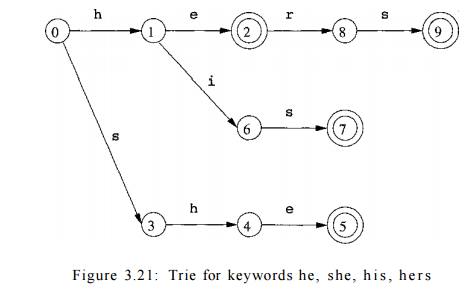
The failure function for the general trie is defined as follows. Suppose
s is the state that corresponds to string &i&2 • • • bn. Then f(s) is
the state that corresponds to the longest proper suffix of &i62 • • -bn
that is also a prefix of some keyword. For example, the failure function for
the trie of Fig. 3.21 is:
! Exercise 3.4.10 : Modify the algorithm of Fig. 3.19 to compute the
failure function for general tries. Hint: The major difference is that we
cannot simply test for equality or inequality of bs+1 and bt+i in lines (4) and
(5) of Fig. 3.19. Rather, from any state there may be several transitions out on
several charac-ters, as there are transitions on both e and i from state 1 in
Fig. 3.21. Any of those transitions could lead to a state that represents the
longest suffix that is also a prefix.
Exercise 3.4.11 : Construct the tries and compute the failure function
for the following sets of keywords:
a) aaa, abaaa, and ababaaa .
b) all , fall , fatal , llama, And lame.
c) pipe , pet , item, temper, And perpetual .
! Exercise 3.4.12 : Show that
your algorithm from Exercise 3.4.10 still runs in time that is linear in the
sum of the lengths of the keywords.
Related Topics