Chapter: Compilers : Principles, Techniques, & Tools : Lexical Analysis
From Regular Expressions to Automata
From Regular Expressions to
Automata
1 Conversion of an NFA to a DFA
2 Simulation of an NFA
3 Efficiency of NFA Simulation
4 Construction of an NFA from a
Regular Expression
5 Efficiency of String-Processing
Algorithms
6 Exercises for Section 3.7
The regular expression is the notation of choice for describing lexical
analyzers and other pattern-processing software, as was reflected in Section
3.5. How-ever, implementation of that software requires the simulation of a
DFA, as in Algorithm 3.18, or perhaps simulation of an NFA. Because an NFA
often has a choice of move on an input symbol (as Fig. 3.24 does oh input a from state 0) or on e (as Fig. 3.26
does from state 0), or even a choice of making a transition on e or on a real
input symbol, its simulation is less straightforward than for a DFA. Thus often
it is important to convert an NFA to a DFA that accepts the same language.
In this section we shall first show how to convert NFA's to DFA's. Then,
we use this technique, known as "the subset construction," to give a
useful algo-rithm for simulating NFA's directly, in situations (other than
lexical analysis) where the NFA-to-DFA conversion takes more time than the direct
simulation. Next, we show how to convert regular expressions to NFA's, from
which a DFA can be constructed if desired. We conclude with a discussion of the
time-space tradeoffs inherent in the various methods for implementing regular
expressions, and see how to choose the appropriate method for your application.
1. Conversion
of an NFA to a DFA
The general idea behind the subset construction is that each state of
the constructed DFA corresponds to a set of NFA states. After reading input
flifl2 • • • Q>n, the DFA is in that state which corresponds to the set of
states that the NFA can reach, from its start state, following paths labeled a1a2 • • • an.
It is possible that the number of DFA states is exponential in the
number of NFA states, which could lead to difficulties when we try to implement
this DFA. However, part of the power of the automaton-based approach to lexical
analysis is that for real languages, the NFA and DFA have approximately the
same number of states, and the exponential behavior is not seen.
Algorithm 3.20: The subset construction of a DFA from an NFA.
INPUT : An NFA JV.
OUTPUT : A DFA D accepting the same language as N.
METHOD : Our algorithm constructs a transition table Dtran for D. Each
state of D is a set of NFA states, and we construct Dtran so D will simulate
"in parallel" all possible moves N can make on a given input string.
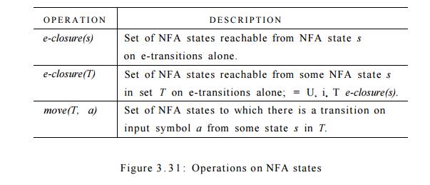
Our first problem is to deal with e-transitions of N properly. In Fig. 3 . 3 1
we see the definitions of several functions that describe basic computations on
the states of N that are needed in the algorithm. Note that s is a single state
of N, while T is a set of states of N.
We must explore those sets of states that N can be in after seeing some input string. As a basis, before
reading the first input symbol, N can
be in any of the states of e-closure(so),
where SQ is its start state. For the
induction, suppose that N can be in
set of states T after reading input
string x. If it next reads input a,
then N can immediately go to any of
the states in move(T, a). However,
after reading a, it may also make several e-transitions; thus N could be in any state of e-closure(move(T, a)) after reading
input xa. Following these ideas, the
construction of the set of Z?'s states, Dstates,
and its transition function Dtran, is
shown in Fig. 3 . 3 2 .
The start state of D is e-closure(so), and the accepting states
of D are all those sets of AT's
states that include at least one accepting state of N. To complete our description of the subset construction, we need
only to show how initially, e-closure(s0) is the only state in Dstates, and it is unmarked;
w h i le ( there is an unmarked state T
in Dstates ) {
mark T;
for ( each input symbol a ) {
U = e-closure(move(T,a));
if ( U is not in Dstates
)
add U as an unmarked state to Dstates;
Dtran[T, a] = U;
}
}
Figure 3.32: The subset construction
e-closure(T) is computed for any set of NFA states
T. This process, shown in Fig.
3.33, is a straightforward search in a graph from a set of states. In this
case, imagine that only the e-labeled edges are available in the graph. •
push all states of T onto stack; initialize e~closure(T) to T; while ( stack is not empty ) {
pop t, the top element, off stack;
for ( each state u
with an edge from t
to u labeled e ) if ( u is not in e-closure(T)
) {
add u to e-closure(T); push u onto
stack;
}
}
Figure 3.33: Computing e-closure(T)
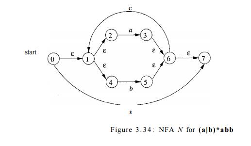
Example 3 . 2 1 : Figure 3.34 shows another NFA accepting (a|b)*abb; it hap-pens to be the one we shall construct directly
from this regular expression in Section 3.7. Let us apply Algorithm 3.20 to
Fig. 3.29.
The start state A of the
equivalent DFA is e-closure(0), or A = {0,1,2,4,7}, since these are exactly
the states reachable from state 0 via a path all of whose edges have label e.
Note that a path can have zero edges, so state 0 is reachable from itself by an
e-labeled path.
The input alphabet is {a, b}. Thus, our first step is to mark A and
compute Dtran[A,a] = e-closure(move(A,a)) and Dtran[A,b] = e-closure(move(A,b)).
Among the states 0, 1, 2, 4, and 7, only 2 and 7 have transitions on a,
to 3 and 8, respectively. Thus, move(A,a) = {3,8} . Also, e-closure({3,8} = { 1
, 2 , 3 , 4 , 6 , 7 , 8 } , so we conclude
Dtran[A,a] = e-closure(move(A,a)) - e-closure({3,8}) = { 1 , 2 , 3 , 4 , 6 , 7 , 8 }
Let us call this set B, so Dtran[A, a] = B.
Now, we must compute Dtran[A,b].
Among the states in A, only 4 has a
transition on 6, and it goes to 5. Thus,
Dtran[A,b] =
e-closure({5}) = { 1 , 2 , 4 , 6 , 7 }
Let us call the above set C, so Dtran[A,
b] — C.
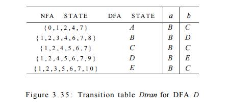
If we continue this process with the unmarked sets B and C, we eventually reach a point where all the states of the
DFA are marked. This conclusion is guaranteed, since there are "only"
2 1 1 different subsets of a set of eleven NFA states. The five different DFA
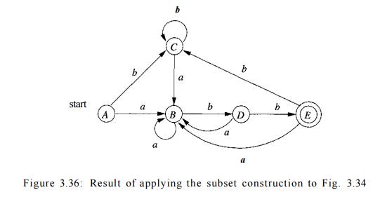
states we actually construct, their correspond-ing sets of NFA states, and the
transition table for the DFA D are
shown in Fig. 3 . 3 5 , and the transition graph for D is in Fig. 3 . 3 6 . State A
is the start state, and state E,
which contains state 10 of the NFA, is the only accepting state.
Note that D has one more state
than the DFA of Fig. 3 . 2 8 for the same lan-guage. States A and C have the same move function, and so can be merged. We discuss the
matter of minimizing the number of states of a DFA in Section 3 . 9 . 6 .
2. Simulation of an NFA
A strategy that has been used in a number of text-editing programs is to
con-struct an NFA from a regular expression and then simulate the NFA using
something like an on-the-fly subset construction. The simulation is outlined
below.
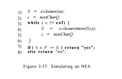
Algorithm 3 . 2 2 : Simulating
an NFA.
INPUT : An input string x
terminated by an end-of-file character
eof. An NFA N with start state SQ, accepting
states F, and transition function move.
OUTPUT : Answer "yes" if M
accepts x; "no"
otherwise.
M E T H O D : The algorithm keeps a set of current states S, those that are reached from
so following a path labeled by the inputs read so far. If c is the next input
character, read by the function nextCharQ,
then we first compute move(S,c) and
then close that set using e-closureQ.
The algorithm is sketched in Fig. 3.37.
3. Efficiency of NFA Simulation
If carefully implemented, Algorithm 3.22 can be quite efficient. As the
ideas involved are useful in a number of similar algorithms involving search of
graphs, we shall look at this implementation in additional detail. The data
structures we need are:
Two stacks, each of which holds a set of NFA states. One of these
stacks, oldStates, holds the "current" set of states, i.e., the value
of S on the right side of line (4) in Fig. 3.37. The second, newStates, holds
the "next" set of states — 5 on the left side of line (4). Unseen is
a step where, as we go around the loop of lines (3) through (6), newStates is
transferred to oldStates.
A boolean array alreadyOn,
indexed by the NFA states, to indicate which states are in newStates. While the
array and stack hold the same infor-mation, it is much faster to interrogate
alreadyOn[s] than to search for state s on the stack newStates. It is for this
efficiency that we maintain both representations.
A two-dimensional array move[s,a]
holding the transition table of the NFA. The entries in this table, which are
sets of states, are represented by linked lists.
To implement line (1) of Fig. 3.37, we need to set each entry in array
alreadyOn to FALSE, then for each state s in e-closure(so), push s onto oldStates
and set alreadyOn[s] to TRUE. This operation on state s, and the implementation
of line (4) as well, are facilitated by a function we shall call addState(s).
This function pushes state s onto newStates, sets alreadyOn[s] to TRUE, and
calls itself recursively on the states in move[s,e] in order to further the
computation of e-closure(s). However, to avoid duplicating work, we must be
careful never to call addState on a state that is already on the stack
newStates. Figure 3.38 sketches this function.
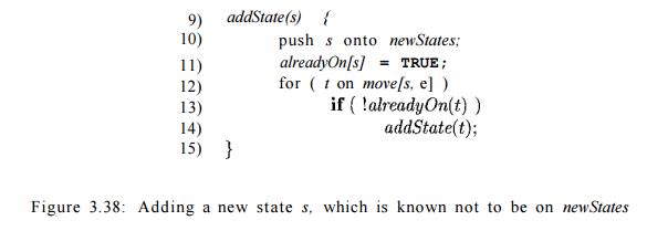
Figure 3.38: Adding a new state
s, which is known not to be on newStates
We implement line (4) of Fig. 3.37 by looking at each state s on
oldStates.
We first find the set of states move[s, c], where c is the next input,
and for each of those states that is not already on newStates, we apply addState to it. Note that addState has the effect
of computing the e- closure and adding all those states to
newStates as well, if they were not already on. This sequence of steps is
summarized in Fig. 3.39.
for ( s o n
oldStates ) {
for ( t on move[s, c] )
if ( \alreadyOn[t]
)
addState(t);
pop s from
oldStates;
}
for ( s on newStates
) {
pop s
from newStates;
push s onto
oldStates;
a/readyOn[s] = FALSE;
}
Figure 3.39: Implementation of step (4) of Fig. 3.37
Now, suppose that the NFA N
has n states and m transitions; i.e., m is
the sum over all states of the number of symbols (or e) on which the state has
a transition out. Not counting the call to addState
at line (19) of Fig. 3.39, the time spent in the loop of lines (16) through
(21) is 0(n). That is, we can go
around the loop at most n times, and each step of the loop requires constant
work, except for the time spent in addState.
The same is true of the loop of lines (22) through (26).
During one execution of Fig. 3.39, i.e., of step (4) of Fig. 3.37, it is
only possible to call addState on a
given state once. The reason is that whenever we call addState(s), we set alreadyOn[s]
to TRUE at line (11) of Fig. 3.39. Once alreadyOn[s]
is TRUE, the tests at line (13) of Fig. 3.38 and line (18) of Fig. 3.39 prevent another call.
The time spent in one call to addState,
exclusive of the time spent in recur-sive calls at line (14), is 0(1) for lines
(10) and (11). For lines (12) and (13), the time depends on how many
e-transitions there are out of state s.
We do not know this number for a given state, but we know that there are at
most m transitions in total, out of all states. As a result, the aggregate time
spent in lines (11) over all calls to addState during one execution of the code
of Fig. 3.39 is 0(m). The aggregate for the rest of the steps of addState is
0(n), since it is a constant per call, and there are at most n calls.
We conclude that, implemented properly, the time to execute line (4) of
Fig. 3.37 is 0(n + m) . The rest of
the while-loop of lines (3) through (6) takes 0(1) time per iteration. If the
input x is of length k, then the total work in that loop is 0((k(n + m ) ) . Line (1) of Fig. 3.37
can be executed in 0 ( n + m) time,
since it is essentially the steps of Fig. 3.39 with oldStates containing only the state so- Lines (2), (7), and (8)
each take 0(1) time. Thus, the running time of Algorithm 3.22, properly
implemented, is 0((k(n + m ) ) . That
is, the time taken is proportional to the length of the input times the size
(nodes plus edges) of the transition graph.
Big-Oh Notation
An expression like 0(n) is a shorthand for "at most some constant
times n." Technically, we say a function / ( n ) , perhaps the running
time of some step of an algorithm, is 0(g(n)) if there are constants c and no,
such that whenever n > n 0 , it is true that / ( n ) < cg(n). A useful
idiom is "0(1)," which means "some constant." The use of
this big-oh notation enables us to avoid getting too far into the details of
what we count as a unit of execution time, yet lets us express the rate at
which the running time of an algorithm grows.
4. Construction of an NFA from a
Regular Expression
We now give an algorithm for converting any regular expression to an NFA
that defines the same language. The algorithm is syntax-directed, in the sense
that it works recursively up the parse tree for the regular expression. For
each subexpression the algorithm constructs an NFA with a single accepting
state.
Algorithm 3 . 2 3 : The McNaughton-Yamada-Thompson algorithm to convert
a regular expression to an NFA.
INPUT : A regular expression r over alphabet S.
OUTPUT : An NFA N accepting L(r).
METHOD : Begin by parsing r into its constituent subexpressions. The rules for constructing an NFA consist of
basis rules for handling subexpressions with no operators, and inductive rules
for constructing larger NFA's from the NFA's for the immediate subexpressions
of a given expression.
BASIS: For expression e construct the NFA
start
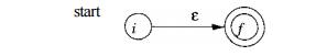
Here, i is a new state, the
start state of this NFA, and / is another new state, the accepting state for
the NFA.
For any subexpression a in S,
construct the NFA
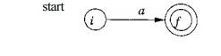
where again i and / are new
states, the start and accepting states, respectively. Note that in both of the
basis constructions, we construct a distinct NFA, with new states, for every
occurrence of e or some o as a subexpression of r.
INDUCTION : Suppose N(s) and N(t) are NFA's for regular expressions s and t, respectively.
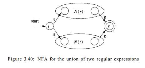
a) Suppose r = s1t. Then N(r), the NFA for r, is constructed as
in Fig. 3.40. Here, i and / are new
states, the start and accepting states of N(r),
respectively. There are e-transitions from i
to the start states of N(s) and N(t), and each of their accepting states
have e-transitions to the accepting state /. Note that the accepting states of N(s) and N(t) are not accepting in N(r).
Since any path from i to / must pass
through either N(s) or N(t) exclusively, and since the label of
that path is not changed by the e's leaving i
or entering /, we conclude that N(r)
accepts L(s) U L(t), which is the same as
L(r). That is, Fig. 3.40 is a correct
construction for the union operator.
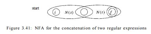
b) Suppose r = st. Then construct N(r) as in Fig. 3.41. The start state
of N(s) becomes the start state of N(r), and the accepting state of N(t) is the
only accepting state of N(r). The accepting state of N(s) and the start state
of N(t) are merged into a single state, with all the transitions in or out of
either state. A path from i to / in Fig. 3.41 must go first through N(s), and
therefore its label will begin with some string in L(s). The path then
continues through N(t), so the path's label finishes with a string in L(t). As
we shall soon argue, accepting states never have edges out and start states
never have edges in, so it is not possible for a path to re-enter N(s) after
leaving it. Thus, N(r) accepts exactly L(s)L(i), and is a correct NFA for r =
st.
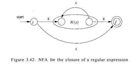
c) Suppose r = s*. Then for r we construct the NFA N(r) shown in Fig.
3.42. Here, i and / are new states, the start state and lone accepting state of
N(r). To get from i to /, we can either follow the introduced path labeled e,
which takes care of the one string in L(s)°, or we can go to the start state of
N(s), through that NFA, then from its accepting state back to its start state
zero or more times. These options allow N(r) to accept all the strings in
L(s)1, L(s)2, and so on, so the entire set of strings accepted by N(r) is
L(s*).
d) Finally, suppose r = (s). Then L(r) = L(s), and we can use the NFA
N(s) as N(r).
The method description in Algorithm 3.23 contains hints as to why the
inductive construction works as it should. We shall not give a formal
correctness proof, but we shall list several properties of the constructed
NFA's, in addition to the all-important fact that N(r) accepts language L(r).
These properties are interesting in their own right, and helpful in making a
formal proof.
N(r) has at most twice as many
states as there are operators and operands in r. This bound follows from the
fact that each step of the algorithm creates at most two new states.
N(r) has one start state and one accepting
state. The accepting state has no outgoing transitions, and the start state has
no incoming transitions.
Each state of N(r) other than the
accepting state has either one outgoing transition on a symbol in E or two
outgoing transitions, both on e.
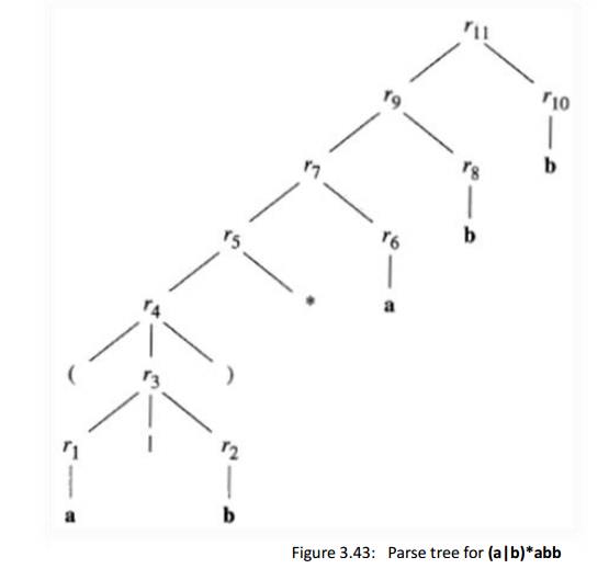
Example 3.24 : Let us use Algorithm 3.23 to construct an NFA for r =
(a|b)*abb . Figure 3.43 shows a parse tree for r that is analogous to the parse
trees constructed for arithmetic expressions in Section 2.2.3. For
subexpression r i , the first a, we construct the NFA:
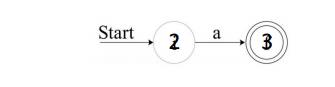
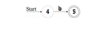
State numbers have been chosen for consistency with what follows. For r2
we construct:
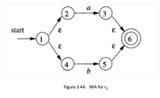
We can now combine JV(n) and N(r2), using the construction of Fig. 3.40
to obtain the NFA for r3 = ri\r2] this NFA is shown in Fig. 3.44.
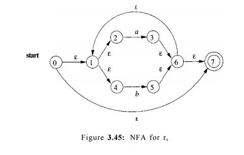
The NFA for r4 = (73) is the same as that for 7-3. The NFA for r5 = (r 3 )* is
then as shown in Fig. 3.45. We have used the construction in Fig. 3.42 to build
this NFA from the NFA in Fig. 3.44.
Now, consider subexpression r§,
which is another a. We use the basis
con-struction for a again, but we
must use new states. It is not permissible to reuse
the NFA we constructed for r1,
even though r1 and r% are the same expression. The NFA for
r 6 is:
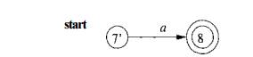
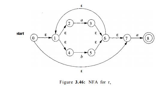
To obtain the NFA for rr = r5re, we apply the construction of Fig. 3.41.
We merge states 7 and 7', yielding the NFA of Fig. 3.46. Continuing in this fashion with
new NFA's for the two subexpressions b
called rg and rio, we eventually
construct the NFA for (a|b)*abb that
we first met in Fig. 3.34. •
5. Efficiency of
String-Processing Algorithms
We observed that Algorithm 3.18
processes a string x in time 0(|a?|), while in Section 3.7.3 we concluded that we could
simulate an NFA in time proportional to the product of \x\ and the size of the NFA's transition graph. Obviously, it is
faster to have a DFA to simulate than an NFA, so we might wonder whether it
ever makes sense to simulate an NFA.
One issue that may favor an NFA is that the subset construction can, in
the worst case, exponentiate the number of states. While in principle, the
number of DFA states does not influence the running time of Algorithm 3.18,
should the number of states become so large that the transition table does not
fit in main memory, then the true running time would have to include disk I / O
and therefore rise noticeably.
Example 3 . 2 5 : Consider the family of languages described by regular expres-sions of
the form Ln — (a|b)*a(a|b)™_ 1 , that is, each language Ln consists of strings of a's and &'s such that the nth character to
the left of the right end holds a. An
n + 1-state NFA is easy to construct. It stays in its initial state under any
input, but also has the option, on input a, of going to state 1. From state 1,
it goes to state 2 on any input, and so on, until in state n it accepts. Figure
3.47 suggests this NFA.
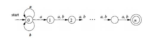
Figure 3.47: An NFA that has many
fewer states than the smallest equivalent DFA
However, any DFA for the language Ln must have at least 2n states. We
shall not prove this fact, but the idea is that if two strings of length n can
get the DFA to the same state, then we can exploit the last position where the
strings differ (and therefore one must have a, the other b) to continue the
strings identically, until they are the same in the last n — 1 positions. The
DFA will then be in a state where it must both accept and not accept.
Fortunately, as we mentioned, it is rare for lexical analysis to involve
patterns of this type, and we do not expect to encounter DFA's with outlandish
numbers of states in practice. •
However, lexical-analyzer generators and other string-processing systems
often start with a regular expression. We are faced with a choice of converting
the regular expression to an NFA or DFA. The additional cost of going to a DFA
is thus the cost of executing Algorithm 3.23 on the NFA (one could go directly
from a regular expression to a DFA, but the work is essentially the same). If
the string-processor is one that will be executed many times, as is the case
for lexical analysis, then any cost of converting to a DFA is worthwhile.
However, in other string-processing applications, such as grep, where
the user specifies one regular expression and one or several files to be
searched for the pattern of that expression, it may be more efficient to skip
the step of constructing a DFA, and simulate the NFA directly.
Let us consider the cost of converting a regular expression r to an NFA
by Algorithm 3 . 2 3 . A key step is constructing the parse tree for r. In
Chapter 4 we shall see several methods that are capable of constructing this
parse tree in linear time, that is, in time 0 ( | r | ) , where |r| stands for
the size of r — the sum of the number of operators and operands in r. It is
also easy to check that each of the basis and inductive constructions of
Algorithm 3 . 2 3 takes constant time, so the entire time spent by the
conversion to an NFA is 0 ( [ r | ) .
Moreover, as we observed in Section 3 . 7 . 4 , the NFA we construct has
at most |r| states and at most 2\r\ transitions. That is, in terms of the
analysis in Section 3 . 7 . 3 , we have n < \r\ and m < 2\r\. Thus,
simulating this NFA on an input string x takes time 0(\r\ x \x\). This time dominates
the time taken by the NFA construction, which is 0 ( | r | ) , and therefore,
we conclude that it is possible to take a regular expression r and string x,
and tell whether x is in L(r) in time 0(\r\ x \x\).
The time taken by the subset construction is highly dependent on the
num-ber of states the resulting DFA has. To begin, notice that in the subset
construction of Fig. 3 . 3 2 , the key step, the construction of a set of
states U from a set of states T and an input symbol a, is very much like the
construction of a new set of states from the old set of states in the NFA
simulation of Algo-rithm 3 . 2 2 . We already concluded that, properly
implemented, this step takes time at most proportional to the number of states
and transitions of the NFA.
Suppose we start with a regular expression r and convert it to an NFA.
This NFA has at most |r| states and at most 2\r\ transitions. Moreover, there
are at most |r| input symbols. Thus, for every DFA state constructed, we must
construct at most |r| new states, and each one takes at most 0(\r\ + 2\r\)
time. The time to construct a DFA of s states is thus 0{\r\2s).
In the common case where s is about |r|, the subset construction takes
time 0(\r\3). However, in the worst case, as in Example 3 . 2 5 , this time is
0(\r\22^). Figure 3 . 4 8 summarizes the options when one is given a regular
expression r and wants to produce a recognizer that will tell whether one or
more strings x are in L(r).
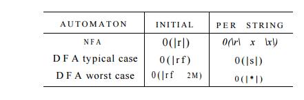
Figure 3 . 4 8 : Initial cost and per-string-cost of various methods of
recognizing the language of a regular expression
If the per-string cost dominates, as it does when we build a lexical
analyzer, we clearly prefer the DFA.
However, in commands like grep, where we run the automaton on only one string,
we generally prefer the NFA. It is not until |x| approaches |r| 3 that we
would even think about converting to a DFA.
There is, however, a mixed strategy that is about as good as the better
of the NFA and the DFA strategy for each expression r and string x. Start off simulating the NFA, but
remember the sets of NFA states (i.e., the DFA states) and their transitions,
as we compute them. Before processing the current set of NFA states and the
current input symbol, check to see whether we have already computed this transition,
and use the information if so.
Related Topics