Economics - Law of Demand | 11th Economics : Chapter 2 : Consumption Analysis
Chapter: 11th Economics : Chapter 2 : Consumption Analysis
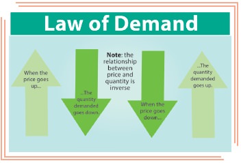
Law of Demand
Law of
Demand
Demand is
essential for the creation, survival and profitability of a firm. “Demand in economics is the desire to possess something and the willingness and
the ability to pay a certain price in order to possess it”.
-J. Harvey
“Demand in
economics means desire backed up by enough money to pay for the good demanded”
1. Characteristics of Demand
Price : Demand is always related to
price.
Time : Demand always means demand per
unit of time, per day, per week, per month
or per year.
Market : Demand is always related to the
market, buyer and sellers.
Amount : Demand is always a specific
quantity which a consumer is willing to purchase.
2. Demand Function
Demand
depends upon price. This means demand for a commodity is a function of price.
Demand function mathematically is denoted as,
D = f (P)
where, D
= Demand, f = function P = Price
3. Law of Demand
The Law
of Demand was first stated by Augustin Cournot in 1838. Later it was refined
and elaborated by Alfred Marshall.
Definitions
The Law
of Demand says as “the quantity demanded increases with a fall in price and
diminishes with a rise in price”.
-Marshall
“The Law
of Demand states that people will buy more at lower price and buy less at
higher prices, other things remaining the same”.
-Samuelson
Assumptions of Law of Demand
1.
The income of the consumer remains constant.
2.
The taste, habit and preference of the consumer
remain the same.
3.
The prices of other related goods should not
change.
4.
There should be no substitutes for the commodity in
study.
5.
The demand for the commodity must be continuous.
6.
There should not be any change in the quality of
the commodity.
Given
these assumptions, the law of demand operates. If there is change even in one
of these assumptions, the law will not operate.
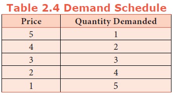
Demand Schedule
Explanation
The law of demand explains the relationship
between the price of a commodity and the quantity demanded of it.
This law states that
quantity demanded of a commodity expands with a fall in price and contracts
with a rise in price. In other words, a rise in price of a commodity is
followed by a contraction demand and a fall in price is followed by extension
in demand. Therefore, the law of demand states that there is an inverse
relationship between the price and the quantity demanded of a commodity.
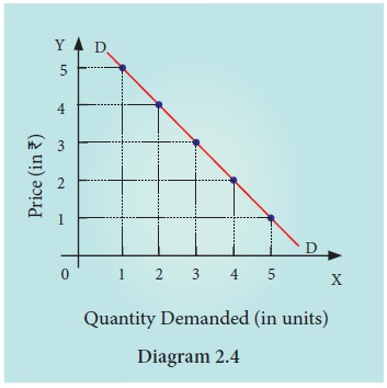
In the
diagram 2.4, X axis represents the quantity demanded and Y axis represents the
price of the commodity.
is the
demand curve, which has a negative slope i.e., slope downward from left to
right which indicates that when price falls, the demand expands and when price
rises, the demand contracts.
Market Demand for a Commodity
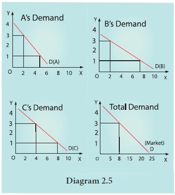
The
market demand curve for a commodity is derived by adding the quantum demanded
of the commodity by all the individuals constituting the market. In the diagram
given above, the final market demand curve represents the addition of the
demand curve of the individuals A, B and C at the same price.
When
Price is Rs.3, the Market demand is
2+2+4 = 8 When Price is Rs.1, the Market
demand is 6+8+8 = 22
As in the
case of individual demand schedule, the Market Demand Curve is at a price, at a
place and at a time.
4. Determinants of Demand
1.
Changes in Tastes and Fashions: The
demand for some goods and services is very susceptible to changes in
tastes and fashions
2.
Changes in Weather: An
unusually dry summer results in a increase in the demand for cool
drinks.
3.
Taxation and Subsidy: If fresh
taxes are levied or the existing rates of taxation on commodities are
increased their prices go up. The subsidies will bring down the prices. Therefore
taxes reduce demand and subsidies raise demand.
4.
Changes in Expectations: Expectations
also bring about a change in demand. Expectation of rise in price in future
results in increase in demand.
5.
Changes in Savings: Savings
and demand are inversely related.
6.
State of Trade Activity: During
the periods of boom and prosperity, the demand for all commodities tends to
increase. On the contrary, during times of depression there is a general
slackening of demand.
7.
Advertisement: In
advanced capitalistic countries advertising is a powerful instrument increasing
the demand in the market.
8.
Changes in Income: An
increase in family income may increase the demand for durables like video
recorders and refrigerators. Equal distribution of income enables poor to get
more income. As a result consumption level increases.
9.
Change in Population: The
demand for goods depends on the size of population. An increase in population
tends to increase the demand for goods and a decrease in population tends to
decrease the demand (if other things remain constant).
5. Exceptions to the law of demand
Normally,
the demand curve slopes downwards from left to right. But there are some
unusual demand curves which do not obey the law and the reverse occurs. A fall
in price brings about a contraction of demand and a rise in price results in an
extension of demand. Therefore the demand curve slopes upwards from left to
right. It is known as exceptional demand curve.
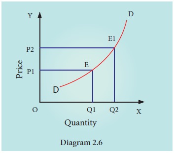
In the
diagram 2.6, DD is the demand curve which slopes upwards from left to right. It
shows that when price is OP1, OQ1 is the demand and when
the price rises to OP2, demand also extends to OQ2.
6. Reasons for Exceptional Demand Curve
1.
Giffen
Paradox: The Giffen good or inferior good is an exception to the law of demand. When the price of an inferior
good falls, the poor will buy less and vice versa.
2.
Veblen or
Demonstration effect: Veblen has explained the exceptional demand curve through his doctrine of
conspicuous consumption. Rich people buy certain goods because it gives social
distinction or prestige. For example, diamonds.
3.
Ignorance: Sometimes,
the quality of the commodity is judged by it’s price. Consumers think that the
product is superior if the price is high. As such they buy more at a higher
price.
4.
Speculative
effect: If the price of the commodity is increasing then the consumers will buy more of it because of the
expectation that it will increase still further. Eg stock markets.
5.
Fear of
shortage: During times of emergency or war, people may expect shortage of a commodity and so buy more.
7. Extension and Contraction of Demand
The changes in the quantity demanded for a commodity due to the change in its price alone are called “Extension and Contraction of Demand”. In other words, buying more at a lower price and less at a higher price is known as “Extension and Contraction of Demand”.
8. Movement along Demand Curve
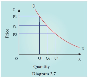
In the
diagram 2.7, at point A, the price OP2 and quantity demanded is OQ2.
When price falls to OP3 (movement along the demand curve A to C) the
quantity demanded increases to OQ3. If price rises to OP1 (movement
from A to B) quantity demanded decreases to OQ1.
9. Shift in the Demand Curve
A shift
in the demand curve occurs with a change in the value of a variable other than
its price in the general demand function. An increase or decrease in demand due
to changes in conditions of demand is shown by way of shifts in the demand
curve.
On the
left hand side of the diagram 2.8, the original demand curve is d1d1,
the price is OP1 and the quantity demanded is OQ1. Due to
change in the conditions of demand (change in income, taste or change in prices
of substitutes and /or complements) the quantity demanded decreases from OQ1
to OQ2. This is shown in the demand curve to the left. The new
demand curve is d1d1. This is called decrease in demand.
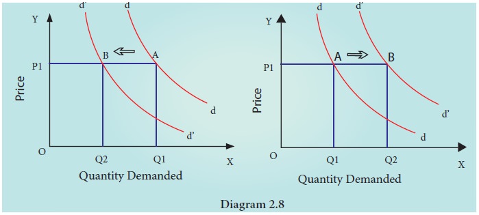
On the
right hand side of the diagram 2.8, the original price is OP1 and
the quantity demanded is OQ1 . Due to changes in other conditions,
the quantity purchased has increased to OQ2 . Thus the demand curve
shifts to the right d1d1. This is called increase in
demand.
‘Extension’
and ‘Contraction’ of demand follow a change in price. Increases and decreases
in demand take place when price remains the same and the other factors bring
about demand changes.
Related Topics