Introduction to Econometrics

Introduction To Econometrics

Origin Of Econometrics

Economists tried to support their ideas with facts and figures in ancient times. Irving Fisher is the first person, developed mathematical equation in the quantity theory of money with help of data. Ragnar Frisch, a Norwegian economist and statistician named the integration of three subjects such that mathematics, statistical methods and economics as Econometrics” in 1926.

The term econometrics is formed from two words of Greek origin, ‘oukovouia’ meaning economy and ‘uetpov’ meaning measure. Econometrics emerged as an independent discipline studying economics phenomena.

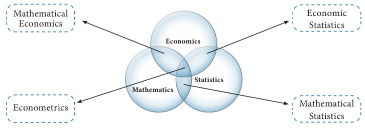
Econometrics may be considered as the integration of economics, Statistics and Mathematics.

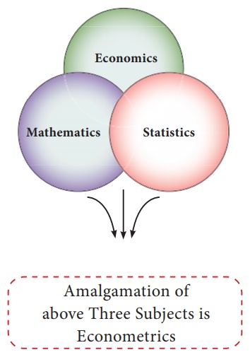
Econometrics is an amalgamation of three subjects which can be easily understood by following Venn diagram and picture representation.

Economics + Mathematics= Mathematical Economics

Mathematical Economics+ Statistical Data & Its Technique = Econometrics

{Economics + Statistics + Mathematics}+Empirical Data = Econometrics

Definitions

In the words of Arthur S. Goldberger, “Econometrics may be defined as the social science in which the tools of economic theory, mathematics and statistical inference are applied to the analysis of economic phenomena”.

Gerhard Tinbergen points out that “Econometrics, as a result of certain outlook on the role of economics, consists of application of mathematical statistics to economic data to lend empirical support to the models constructed by mathematical economics and to obtain numerical results”.

H Theil “Econometrics is concerned with the empirical determination of economic laws”

In the words of Ragnar Frisch “The mutual penetration of quantitative econometric theory and statistical observation is the essence of econometrics”.

Econometrics means economic measurement. Econometrics deals with the measurement of economic relationships.

Objectives Of Econometrics

The general objective of Econometrics is to give empirical content to economic theory.

The specific objectives are as follows:

1.        It helps to explain the behaviour of a forthcoming period that is forecasting economic phenomena.

2.        It helps to prove the old and established relationships among the variables or between the variables

3.        It helps to establish new theories and new relationships.

4.        It helps to test the hypotheses and estimation of the parameter.

Methodology Of Econometrics

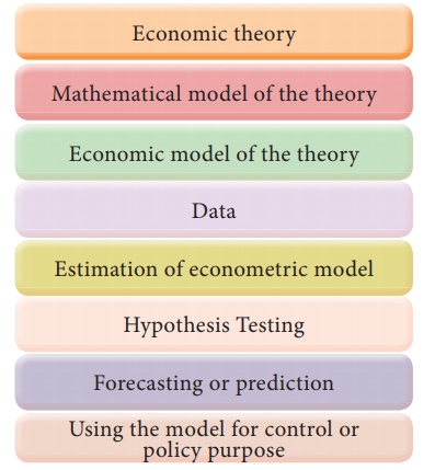
Broadly speaking, traditional or classical econometric methodology consists of the following steps.

1.        Statement of the theory or hypothesis

2.        Specification of the mathematical model of the theory

3.        Specification of the econometric model of the theory

4.        Obtaining the data

5.        Estimation of the parameters of the econometric model

6.        Hypothesis testing

7.        Forecasting or prediction

8.        Using the model for control or policy purposes.

Flow Chart of Anatomy / Methodology of Econometrics

Anatomy of Econometric Modeling

Difference between the Econometric model with Mathematical models and statistical models

1. Models in Mathematical Economics are developed based on Economic Theories, while, Econometric Models are developed based on Economic Theories to test the validity of Economic Theories in reality through the actual data.

2. Regression Analysis in Statistics does not concentrate more on error term while Econometric Models concentrate more on error terms

Statistics Regression:

Yi = β₀ + β₁X_i

Econometrics Regression:

Yi = β₀ + β₁X_i+ U_i

(with more than 2 variables) or Y = β₀ + β₁X₁ + β₂X₂ + β₃X₃+U_i

Systematic Part: β₀ + β₁Xi or explained part and Random Part: U_i unexplained part in a regression. U_i represents the role of omitted variables in specifying a regression relationship of Y on X. Hence, the U_i cannot and should not be ignored.

Assumptions of the Linear Regression Model

The Linear regression model is based on certain assumptions

1.        Some of them refer to the distribution of the random variable .

2.        Some of them refer to the relationship between U_i and the explanatory variables (x₁, x₂, x₃ given in the above example).

3.        Some of them refer to the relationship between U_i the explanatory variables themselves.

Assumptions about the distribution of the values of are called stochastic assumptions of ordinary least squares (OLS). Assumptions relating to the relationship between U_i and explanatory variables and relating to the relationship among the explanatory variables are called other assumptions.

Assumptions

1.        "U" is a random real variable. That is "U" may assume positive, negative or zero values. Hence the mean of the "U" will be zero.

2.        The variance of "U" is constant for all values of "U"

3.        The "U" has a normal distribution.

4.        The Covariances of any U_i with any other U_j are equal to zero

5.        "U" is independent of explanatory variable (s)

6.        Explanatory variables are measured without error.

7.        The explanatory variables are not perfectly linearly correlated.

8.        The variables are correctly aggregated.

9.        The relationship is correctly identified and specified.

10.   Parameters are linear.