Correlation

Correlation

Introduction

Correlation  is  a  statistical  device that helps to analyse the covariation of two or more variables. Sir Francis Galton,is  responsible for  the calculation of correlation coefficient.

Types of Correlation

Correlation is classified in   several different ways. Three of the most important ways of classifying correlation are

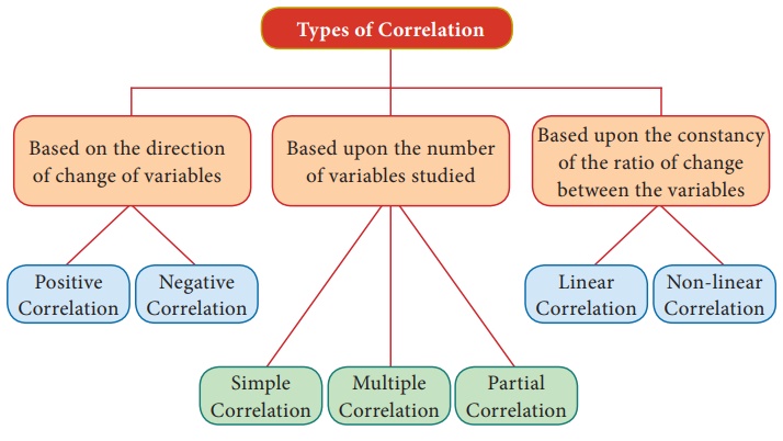
Type I: Based on the direction of change of variables

Correlation is classified into two types as Positive correlation and Negative Correlation based on the direction of change of the variables.

i. Positive Correlation:

The correlation is said to be positive if the values of two variables move in the same direction.

Ex 1: If income and Expenditure of a Household may be increasing or decreasing simultaneously. If so, there is positive correlation. Ex. Y= a + bx

ii. Negative Correlation:

The Correlation is said to be negative when the values of variables move in the opposite directions. Ex. Y= a – bx

Ex 1: Price and demand for a commodity move in the opposite direction.

Type II: Based upon the number of variables studied.

There are three types based upon the number of variables studied as

i) Simple Correlation

ii) Multiple Correlation

iii) Partial Correlation

i) Simple Correlation:

If only two variables are taken for study then it is said to be simple correlation. Ex. Y= a + bx

ii) Multiple Correlations:

If three or more than three variables are studied simultaneously, then it is termed as multiple correlation.

Ex: Determinants of Quantity demanded

Q_d= f (P, Pc, Ps, t, y)

Where Q_d stands for Quantity demanded, f stands for function.

P is the price of the goods,

P_c is the price of competitive goods

P_s is the price of substituting goods

t is the taste and preference

y is the income.

iii) Partial Correlation:

If there are more than two variables but only two variables are considered keeping the other variables constant, then the correlation is said to be Partial Correlation

Type III: Based upon the constancy of the ratio of change between the variables

Correlation is divided into two types as linear correlation and Non-Linear correlation based upon the Constancy of the ratio of change between the variables.

i) Linear Correlation: Correlation is said to be linear when the amount of change in one variable tends to bear a constant ratio to the amount of change in the other.

Ex. Y= a + bx

ii) Non Linear: The correlation would be non -linear if the amount of change in one variable does not bear a constant ratio to the amount of change in the other variables.

Ex. Y= a + bx2

Methods of Studying Correlation:

The various methods of ascertaining whether two variables are correlated or not are:

1. Scatter diagram Method

2. Graphic Method

3. Karl Pearson’s Co - efficient of correlation and

4. Method of Least Squares.

Of these, the first two are based on the knowledge of diagram and graphs, whereas the others are mathematical methods.

1. Scatter Diagram Method:

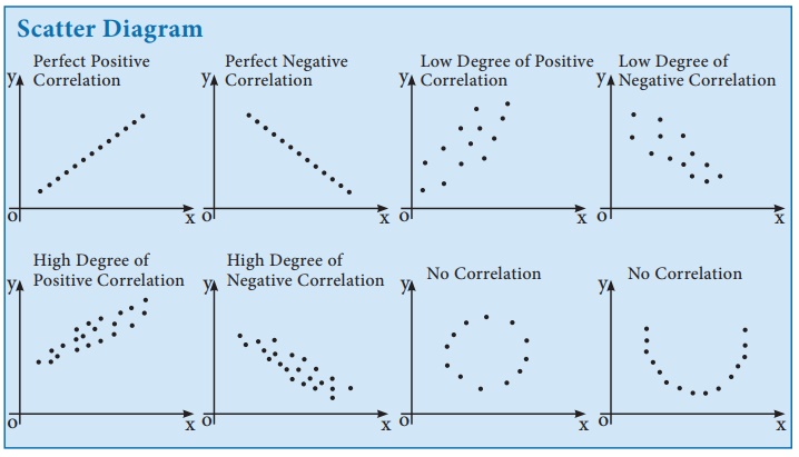
Scatter diagram is a graph of observed plotted points where each point represents the values of X and Y as a coordinate. It portrays the relationship between these two variables graphically.

Advantages of Scatter Diagram method

(1) It is very simple and non- mathematical method

(2) it is not influenced by the size of extreme item.

(3) It is the first step in resting the relationship between two variables.

Disadvantages of Scatter diagram method

It cannot establish the exact degree of correlation between the variables, but provides direction of correlation and depicts it is high or low.

2. Graphic method

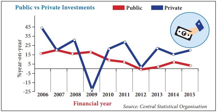
In this method, the individual values of two variables are plotted on the graph sheet and draw the curves of both the variables say x and y. If both X and Y are moving in the same direction either upward or downward, then the correlation is said to be positive. If the curves of X and Y move in the opposite direction; then the correlation is said to be negative.

3. Karl Pearson’s Coefficient of Correlation

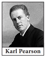
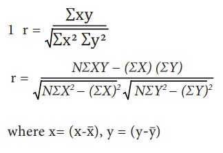
Karl Pearson’s Method is popularly known as Pearson’s coefficient of correlation denoted by the symbol ‘r’. The coefficient of correlation ‘r’ measures the degree of linear relationship between two variables say X and Y. The Formula for computing Karl Pearson’s Coefficient of correlation is:

1) 

‘r’ is calculated by Direct Method without taking deviation of terms either from actual mean or assumed mean.

2) r is calculated by taking the Deviation from actual mean.

3) ‘r’ is calculated by taking assumed mean

Where dx refers to deviations of x series from assumed mean (x x̅), dy refers to deviations of y series from an assumed mean of (y-y) y

∑dxdy =  Sum of product of the deviations x and y series from their assumed means.

∑dx² = Sum of the squares of the deviations of X series from an assumed mean

∑dy²= Sum of the squares of the deviations  of x series from an assumed mean

∑dx = sum of the deviation of x series  from an assumed mean of x

∑dy = sum of the deviation of y series from an assumed mean of y

Procedure for Computing the Correlation Coefficient: (For Direct and Deviation from actual mean method).

Step-1 Calculate the mean of two series ‘X’’Y’

Step-2 Calculate the deviations ‘X’ and Y in two series from their respective mean.

Step-3 Square each deviations of ‘X’ and ‘Y’ then obtain the sum of the Squared deviation, That is and

Step-4 Multiply each deviation under X with each deviation under Y and obtain the product of ‘xy’. Then obtain the sum of the product of X,Y. Then obtain the sum of the product of x,y is ∑xy.

Step-5 Substitute the value in the formula.

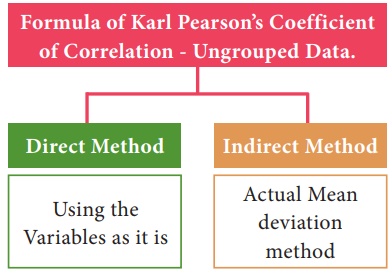
2. Assumed Mean Deviation Method

2. Indirect Method

Indirect Method

dx= (x-x̅) and dy = (y-y̅)

r is free from origin

r is free from unit of measurement -1≤r≤+1

Direct Method:

Example 1: Calculate Karl Pearson’s Coefficient of correlation from the following data and interpret its value:

Price :X 10 12 14 15 19

Supply:Y 40 41 48 60 50

Solution: Let us take Price as X and supply as Y

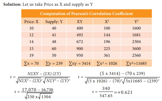
Price of the product and supply for the product is positively correlated. When price of the product increases then the supply for the product also increases.

Actual Mean Method:

Ex-1: Estimate the coefficient of correlation with actualmean method for the following data.

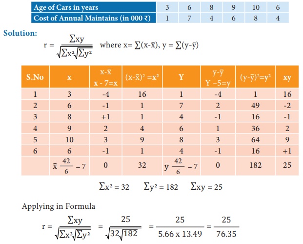
r = 0.327, The Car is getting old in years the cost of maintenance is also increasing. The age of Car and its maintenance are positively correlated.

Assumed Mean Deviation Method

Ex 1: Find the Karl Pearson coefficient of Correlation between X and Y from the following data:

X: 10 12 13 16 17 20 25

Y: 19 22 26 27 29 33 37

Solution:

Formula for Assumed Mean Deviation method.

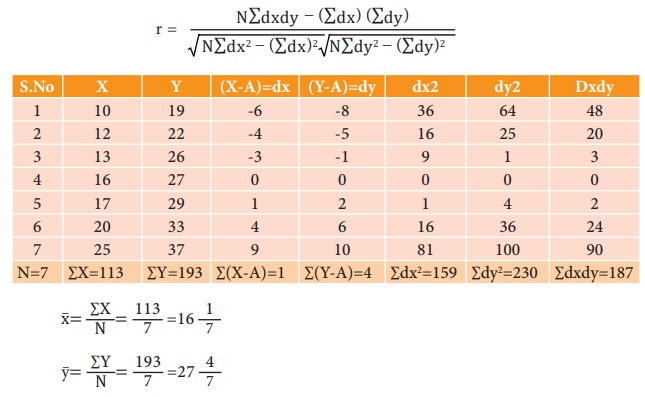
Take the assumed values A = 16 & B = 27 therefore dx = X – A ⇒X – 16 and

∴ dy = Y- A ⇒ Y – 27

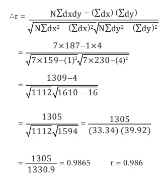
There exists a positive high correlation between X and Y