Improvements to the Pipelining Algorithms

9. Improvements to the Pipelining Algorithms

Algorithm 10.21 is a rather simple algorithm, although it has been found to work well on actual machine targets. The important elements in this algorithm are

1.         The use of a modular resource-reservation table to check for resource conflicts in the steady state.

2.          The need to compute the transitive dependence relations to find the legal range in which a node can be scheduled in the presence of dependence cycles.

3.          Backtracking is useful, and nodes on critical cycles (cycles that place the highest lower bound on the initiation interval T) must be rescheduled together because there is no slack between them.

There are many ways to improve Algorithm 10.21. For instance, the al-gorithm takes a while to realize that a 3-clock initiation interval is infeasible for the simple Example 10.22. We can schedule the strongly connected com-ponents independently first to determine if the initiation interval is feasible for each component.

We can also modify the order in which the nodes are scheduled. The order used in Algorithm 10.21 has a few disadvantages. First, because nontrivial SCC's are harder to schedule, it is desirable to schedule them first. Second, some of the registers may have unnecessarily long lifetimes. It is desirable to pull the definitions closer to the uses. One possibility is to start with scheduling strongly connected components with critical cycles first, then extend the schedule on both ends.

10. Modular Variable Expansion

A scalar variable is said to be privatizable in a loop if its live range falls within an iteration of the loop. In other words, a privatizable variable must not be live upon either entry or exit of any iteration. These variables are so named because different processors executing different iterations in a loop can have their own private copies and thus not interfere with one another.

Variable expansion refers to the transformation of converting a privatizable scalar variable into an array and having the ith iteration of the loop read and write the ith element. This transformation eliminates the antidependence con-straints between reads in one iteration and writes in the subsequent iterations, as well as output dependences between writes from different iterations. If all loop-carried dependences can be eliminated, all the iterations in the loop can be executed in parallel.

Eliminating loop-carried dependences, and thus eliminating cycles in the data-dependence graph, can greatly improve the effectiveness of software pipe-lining. As illustrated by Example 10.15, we need not expand a privatizable variable fully by the number of iterations in the loop. Only a small number of iterations can be executing at a time, and privatizable variables may simultane-ously be live in an even smaller number of iterations. The same storage can thus be reused to hold variables with nonoverlapping lifetimes. More specifically, if the lifetime of a register is I clocks, and the initiation interval is T, then only Q = I T I values can be live at any one point. We can allocate q registers to the variable, with the variable in the ith iteration using the  (i mod q)th register.  We refer to this  transformation as modular variable expansion.

Algorithm 10 . 23 :  Software pipelining with modular variable expansion.

INPUT : A data-dependence graph and a machine-resource description.

OUTPUT : Two loops, one software pipelined and one unpipelined.

M E T H O D :

1.         Remove the loop-carried antidependences and output dependences asso-ciated with privatizable variables from the data-dependence graph.

2.         Software-pipeline the resulting dependence graph using Algorithm 10.21.

Let T be the initiation interval for which a schedule is found, and L be

the length of the schedule for one iteration.

3. From the resulting schedule, compute q_v, the minimum number of regis-ters needed by each privatizable variable v. Let Q = max _w q_v.

4.        Generate two loops: a software-pipelined loop and an unpipelined loop. The software-pipelined loop has

copies of the iterations, placed T clocks apart.  It has a prolog with

instructions, a steady state with QT instructions, and an epilog of L — T instructions. Insert a loop-back instruction that branches from the bottom of the steady state to the top of the steady state.

The number of registers assigned to privatizable variable v is

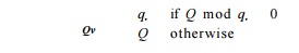
The variable v in iteration i uses the (i mod q'^th register assigned.

Let n be the variable representing the number of iterations in the source loop. The software-pipelined loop is executed if

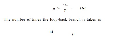
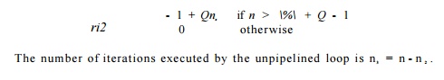
Thus, the number of source iterations executed by the software-pipelined loop is

E x a m p l e 1 0 . 2 4 : For the software-pipelined loop in Fig. 10.22, L = 8, T — 2, and Q = 2. The software-pipelined loop has 7 copies of the iterations, with the prolog, steady state, and epilog having 6, 4, and 6 instructions, respectively. Let n be the number of iterations in the source loop. The software-pipelined loop is executed if n > 5, in which case the loop-back branch is taken

of the iterations in the source loop.  

Modular expansion increases the size of the steady state by a factor of Q. Despite this increase, the code generated by Algorithm 10.23 is still fairly compact. In the worst case, the software-pipelined loop would take three times as many instructions as that of the schedule for one iteration. Roughly, together with the extra loop generated to handle the left-over iterations, the total code size is about four times the original. This technique is usually applied to tight inner loops, so this increase is reasonable.

Algorithm 10.23 minimizes code expansion at the expense of using more registers. We can reduce register usage by generating more code. We can use the minimum q_v registers for each variable v if we use a steady state with

instructions. Here, LCM_V represents the operation of taking the least common multiple of all the q_v's, as v ranges over all the privatizable variables (i.e., the smallest integer that is an integer multiple of all the (fo's). Unfortunately, the least common multiple can be quite large even for a few small <^'s.

11. Conditional Statements

If predicated instructions are available, we can convert control-dependent in-structions into predicated ones. Predicated instructions can be software-pipe-lined like any other operations. However, if there is a large amount of data-dependent control flow within the loop body, scheduling techniques described in Section 10.4 may be more appropriate.

If a machine does not have predicated instructions, we can use the concept of hierarchical reduction, described below, to handle a small amount of data-dependent control flow. Like Algorithm 10.11, in hierarchical reduction the control constructs in the loop are scheduled inside-out, starting with the most deeply nested structures. As each construct is scheduled, the entire construct is reduced to a single node representing all the scheduling constraints of its com-ponents with respect to the other parts of the program. This node can then be scheduled as if it were a simple node within the surrounding control construct. The scheduling process is complete when the entire program is reduced to a single node.

In the case of a conditional statement with "then" and "else" branches, we schedule each of the branches independently. Then:

1. The constraints of the entire conditional statement are conservatively taken to be the union of the constraints from both branches.

2. Its resource usage is the maximum of the resources used in each branch.

3.          Its precedence constraints are the union of those in each branch, obtained by pretending that both branches are executed.

This node can then be scheduled like any other node. Two sets of code, cor-responding tp the two branches, are generated. Any code scheduled in parallel with the conditional statement is duplicated in both branches. If multiple con-ditional statements are overlapped, separate code must be generated for each combination of branches executed in parallel.

12. Hardware Support for Software Pipelining

Specialized hardware support has been proposed for minimizing the size of software-pipelined code. The rotating register file in the Itanium architecture is one such example. A rotating register file has a base register, which is added to the register number specified in the code to derive the actual register accessed. We can get different iterations in a loop to use different registers simply by changing the contents of the base register at the boundary of each iteration. The Itanium architecture also has extensive predicated instruction support. Not only can predication be used to convert control dependence to data dependence but it also can be used to avoid generating the prologs and epilogs. The body of a software-pipelined loop contains a superset of the instructions issued in the prolog and epilog. We can simply generate the code for the steady state and use predication appropriately to suppress the extra operations to get the effects of having a prolog and an epilog.

While Itanium's hardware support improves the density of software-pipe-lined code, we must also realize that the support is not cheap. Since software pipelining is a technique intended for tight innermost loops, pipelined loops tend to be small anyway. Specialized support for software pipelining is warranted principally for machines that are intended to execute many software-pipelined loops and in situations where it is very important to minimize code size.

13. Exercises for Section 10.5

Exercise 1 0 . 5 . 1 : In Example 10.20 we showed how to establish the bounds on the relative clocks at which b and c are scheduled. Compute the bounds for each of five other pairs of nodes (i) for general T (ii) for T = 3 (in) for T = 4.

Exercise 10 . 5 . 2 : In Fig. 10.31 is the body of a loop. Addresses such as a(R9) are intended to be memory locations, where a is a constant, and R9 is the register that counts iterations through the loop. You may assume that each iteration of the loop accesses different locations, because R9 has a different value. Using the machine model of Example 10.12, schedule the loop of Fig. 10.31 in the following ways:

a)          Keeping each iteration as tight as possible (i.e., only introduce one nop af-ter each arithmetic operation), unroll the loop twice. Schedule the second

iteration to commence at the earliest possible moment without violat-ing the constraint that the machine can only do one load, one store, one arithmetic operation, and one branch at any clock.

b) Repeat part (a), but unroll the loop three times. Again, start each itera-tion as soon as you can, subject to the machine constraints.

c) Construct fully pipelined code subject to the machine constraints. In this part, you can introduce extra nop's if needed, but you must start a new iteration every two clock ticks.

Exercise 10 . 5 . 3: A certain loop requires 5 loads, 7 stores, and 8 arithmetic operations. What is the minimum initiation interval for a software pipelining of this loop on a machine that executes each operation in one clock tick, and has resources enough to do, in one clock tick:

a)         3 loads, 4 stores, and 5 arithmetic operations.

b)         3 loads, 3 stores, and 3 arithmetic operations.

Exercise 10.5.4: Using the machine model of Example 10.12, Find the min-imum initiation interval and a uniform schedule for the iterations, for the fol-lowing loop:

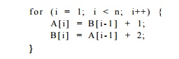
Remember that the counting of iterations is handled by auto-increment of reg-isters, and no operations are needed solely for the counting associated with the for-loop.

!   Exercise 10.5.5 : Prove that Algorithm 10.19, in the special case where every operation requires only one unit of one resource, can always find a software-pipeline schedule meeting the lower bound.

!   Exercise 10.5.6: Suppose we have a cyclic data-dependence graph with nodes

a, b, c, and d. There are edges from a to b and from c to d with label (0,1) and there are edges from b to c and from d to a with label (1,1). There are no other edges.

a)              Draw the cyclic dependence graph.

b)              Compute the table of longest simple paths among the nodes.

c)    Show the lengths of the longest simple paths if the initiation interval T is 2.

d)             Repeat  (c)  if T = 3.

e)              For T = 3, what are the constraints on the relative times that each of the

instructions represented by a, b, c, and d may be scheduled?

 Exercise 10.5.7:  Give an 0 ( n ³ )  algorithm to find the length of the longest simple path in an n-node graph, on the assumption that no cycle has a positive length. Hint: Adapt Floyd's algorithm for shortest paths (see, e.g., A. V. Aho and J. D. Ullman, Foundations of Computer Science, Computer Science Press, New York, 1992).

Exercise 10.5.8: Suppose we have a machine with three instruction types, which we'll call A, B, and C. All instructions require one clock tick, and the machine can execute one instruction of each type at each clock. Suppose a loop consists of six instructions, two of each type. Then it is possible to execute the loop in a software pipeline with an initiation interval of two. However, some sequences of the six instructions require insertion of one delay, and some require insertion of two delays.  Of the 90 possible sequences of two A's, two B's and two C's, how many require no delay?  How many require one delay?

Hint: There is symmetry among the three instruction types so two sequences that can be transformed into one another by permuting the names A, B, and C must require the same number of delays. For example, ABBCAC must be the same as BCCABA.

Summary of Chapter 10

4- Architectural Issues: Optimized code scheduling takes advantage of fea-tures of modern computer architectures. Such machines often allow pipe-lined execution, where several instructions are in different stages of exe-cution at the same time. Some machines also allow several instructions to begin execution at the same time.

4- Data Dependences: When scheduling instructions, we must be aware of the effect instructions have on each memory location and register. True data dependences occur when one instruction must read a location after another has written it. Antidependences occur when there is a write after a read, and output dependences occur when there are two writes to the same location.

•               Eliminating Dependences: By using additional locations to store data, antidependences and output dependences can be eliminated. Only true dependences cannot be eliminated and must surely be respected when the code is scheduled.

•                Data-Dependence Graphs for Basic Blocks: These graphs represent the timing constraints among the statements of a basic block. Nodes corre-

spond to the statements. An edge from n to m labeled d says that the instruction m must start at least d clock cycles after instruction n starts.

 Prioritized Topological Orders: The data-dependence graph for a basic block is always acyclic, and there usually are many topological orders consistent with the graph. One of several heuristics can be used to select a preferred topological order for a given graph, e.g.,  choose nodes with the longest critical path first.

• List Scheduling: Given a prioritized topological order for a data-depend-ence graph, we may consider the nodes in that order. Schedule each node at the earliest clock cycle that is consistent with the timing constraints im-plied by the graph edges, the schedules of all previously scheduled nodes, and the resource constraints of the machine.

• Interblock Code Motion: Under some circumstances it is possible to move statements from the block in which they appear to a predecessor or suc-cessor block. The advantage is that there may be opportunities to execute instructions in parallel at the new location that do not exist at the orig-inal location. If there is not a dominance relation between the old and new locations, it may be necessary to insert compensation code along certain paths, in order to make sure that exactly the same sequence of instructions is executed, regardless of the flow of control.

• Do-All Loops: A do-all loop has no dependences across iterations, so any iterations may be executed in parallel.

• Software Pipelining of Do-All Loops: Software pipelining is a technique for exploiting the ability of a machine to execute several instructions at once. We schedule iterations of the loop to begin at small intervals, per-haps placing no-op instructions in the iterations to avoid conflicts between iterations for the machine's resources. The result is that the loop can be executed quickly, with a preamble, a coda, and (usually) a tiny inner loop.

•              Do-Across Loops: Most loops have data dependences from each iteration to later iterations. These are called do-across loops.

•              Data-Dependence Graphs for Do-Across Loops: To represent the depen-dences among instructions of a do-across loop requires that the edges be labeled by a pair of values: the required delay (as for graphs representing basic blocks) and the number of iterations that elapse between the two instructions that have a dependence.

•              List Scheduling of Loops: To schedule a loop, we must choose the one schedule for all the iterations, and also choose the initiation interval at which successive iterations commence. The algorithm involves deriving the constraints on the relative schedules of the various instructions in the loop by finding the length of the longest acyclic paths between the two nodes. These lengths have the initiation interval as a parameter, and thus put a lower bound on the initiation interval.